HW1. Pet Edge Detection
Topics: Edge detection, Convolution
Problem: Edge detection
As you know, this course is largely funded by grants from Petco,Inc.™ Unfortunately, one of the strings attached to this funding is that we must occasionally assign sponsored problems that cover topics with significant business implications for our sponsor. Our partners at Petco see an opportunity to use computer vision to pull ahead of their bitter rivals, Petsmart™. Instead of painstakingly marking the edges of dogs and cats in pictures by hand—the current industry practice—they have turned to us for an automated solution.
(a) Convolution by the gradient filters
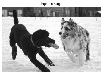
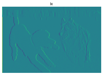
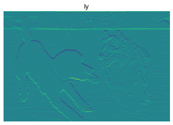
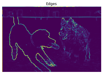
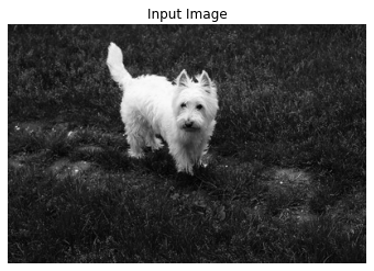
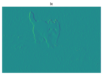
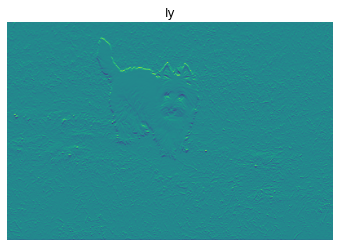
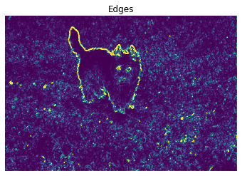
Using the starter code provided, apply the horizontal and vertical gradient filters [1 -1] and [1 − 1]⊤ to the picture of the provided pet producing filter responses $I_x$ and $I_y$. Write a function convolve(im, h) that takes a grayscale image and a 2D filter as input, and returns the result after convolution. Please do not use any “black-box” filtering functions for this, such as the ones in scipy. You may use numpy.dot, but it is not necessary. Instead, implement the convolution as a series of nested for loops. Compute the edge strength as $I_x ^ 2 + I_y ^ 2$. After that, create visualizations of $I_x$, $I_y$, and the edge strength, following the sample code.
The filter response that your function returns should be the same dimensions as the input image. Please use zero padding, i.e. assume that out-of-bounds pixels in the image are zero. Also please make sure to implement convolution, not cross-correlation. Note that this simple filtering method will have a fairly high error rate — there will be true object boundaries it misses and spurious edges that it erroneously detects. The team at Petco, thankfully, has volunteered to painstakingly fix any errors by hand.
import numpy as np, matplotlib as mpl, matplotlib.pyplot as plt, urllib, os
import scipy.ndimage # For image filtering
import imageio # For loading images
import urllib.request
import math

# Download the images that you'll need
base_url = 'https://web.eecs.umich.edu/~ahowens/eecs442/fa20/psets/ps1/ims'
for name in ['dog-1.jpg', 'dog-2.jpg', 'apple.jpg']:
  with open(name, 'wb') as out:
    url = os.path.join(base_url, name)
    out.write(urllib.request.urlopen(url).read())
# You can upload images yourself or load them from URLs
im = imageio.imread('dog-1.jpg')
# Convert to grayscale. We'll use floats in [0, 1].
im = im.mean(2)/255.

# Your code here!
######################### Solution code #########################
def convolve(image, filter):
  output_image = np.zeros(image.shape)

  h, w = image.shape
  k_h, k_w = filter.shape

  p_w = math.ceil((k_w - 1) / 2)
  p_h = math.ceil((k_h - 1) / 2)

  image_padding = np.pad(image, ((p_h, p_h),(p_w, p_w)))

  filter_flip = np.flip(filter)

  for i in range(image_padding.shape[0]):
    for j in range(image_padding.shape[1]):
      if (i >= output_image.shape[0]) or (j >= output_image.shape[1]):
        pass
      else:
        output_image[i,j] = np.sum(np.multiply(image_padding[i:i+k_h, j:j+k_w], filter_flip))


  return output_image

dx = np.array([[1, -1]])
dy = np.array([[1],[-1]])
######################### End solution code #########################

# Convolve the image with horizontal and vertical gradient filters
Ix = convolve(im, dx)
Iy = convolve(im, dy)
edges = Ix**2. + Iy**2.

# Visualize edge maps using matplotlib
plt.figure()
plt.title('Input image')
plt.axis('off')
plt.imshow(im, cmap = 'gray', vmin = 0, vmax = 1)

plt.figure()
plt.axis('off')
plt.title('Ix')
plt.imshow(Ix)

plt.figure()
plt.title('Iy')
plt.axis('off')
plt.imshow(Iy)

plt.figure()
plt.title('Edges')
plt.axis('off')
# Please visualize edge responses using this range of values.
plt.imshow(edges, vmin = 0., vmax = np.percentile(edges, 99))
<matplotlib.image.AxesImage at 0x7f84fc8ccd10>
(b) Image blurring by Gaussian and box filters
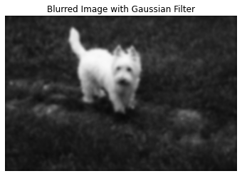
While the edge detector you submitted works well on some pets, engineers are reporting a large number of failures, and Petco higher ups are not happy. Rumor is that it’s failing on pets that are playing in grass, especially for dogs with fluffy coats, such as “doodle” mixes — a particularly lucrative market for our sponsor. It appears that the gradient filter is firing on small, spurious edges.Kindly address our funders’ problem by creating an edge detector that only responds to edges at larger spatial scales. Do this by first blurring the image with a Gaussian filter, before computing gradients. Implement your Gaussian filter on your own. Please do not use any “black-box” Gaussian filter function for this, such as scipy.ndimage.gaussian filter. Apply both the Gaussian filter and the gradient filter using a black-box convolution function scipy.ndimage.convolve on the image, rather than your hand-crafted solution.
(i) Compute the edges without blurring, so we can look at the before-and-after results.
(ii) Compute the blurred image using $\sigma = 2$ and an 11 × 11 Gaussian filter.
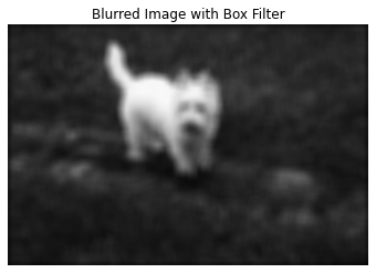
(iii) Instead of blurring the image with a Gaussian filter, use a box filter (i.e., set each of the
11 × 11 filter values to $\frac{1}{11 ^ 2}$).
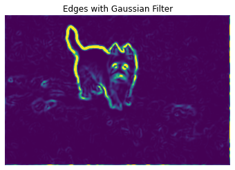
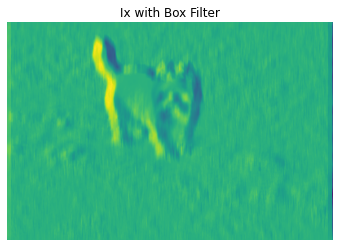
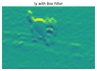
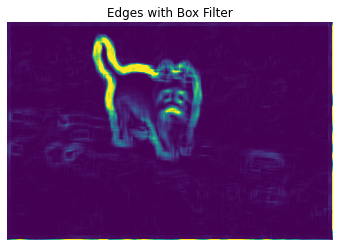
(iv) Compute edges on the two blurred images.
(v) (Optional) Do you see artifacts in the box-filtered result? Describe how the two results
differ. Include your written response in the notebook.
Visualize the edges in the same manner as Problem (a). Your notebook should contain edges that were computed using no blurring, Gaussian blurring, and box filtering. Please also show the two blurred images.
im = imageio.imread('dog-2.jpg').mean(2)/255.
# Your code here!
######################### Solution code #########################
def calculate_gaussian_value(x, y, sigma):
x1 = 2 * np.pi * (sigma**2)
x2 = np.exp(-(x**2 + y**2) / (2 * sigma **2))
return (1 / x1) * x2
def make_gaussian_filter(sigma, n):
gaussian_filter = np.zeros((n, n))
for i in range(gaussian_filter.shape[0]):
for j in range(gaussian_filter.shape[1]):
gaussian_filter[i, j] = calculate_gaussian_value(i - n//2, j - n//2, sigma)
gaussian_filter /= np.sum(gaussian_filter)
return gaussian_filter
def make_box_filter(n):
box_filter = np.ones((n, n))
box_filter *= (1 / n**2)
return box_filter
### Edges without blurring ###
print("====== Edge without blurring ======")
print("")
Ix = scipy.ndimage.convolve(im, dx, mode = "constant", cval = 0)
Iy = scipy.ndimage.convolve(im, dy, mode = "constant", cval = 0)
edges = Ix**2. + Iy**2.
plt.figure()
plt.axis('off')
plt.title('Input Image')
plt.imshow(im, cmap = 'gray', vmin = 0, vmax = 1)
plt.figure()
plt.axis('off')
plt.title('Ix')
plt.imshow(Ix)
plt.figure()
plt.title('Iy')
plt.axis('off')
plt.imshow(Iy)
plt.figure()
plt.title('Edges')
plt.axis('off')
plt.imshow(edges, vmin = 0., vmax = np.percentile(edges, 99))
plt.show()
### Edges with blurred image with gaussian filter ###
print("")
print("====== Edge with blurring by gaussian filter ======")
print("")
gaussian_filter = make_gaussian_filter(sigma = 2, n = 11)
im_blurred_gaussian = scipy.ndimage.convolve(im, gaussian_filter, mode = "constant", cval = 0)
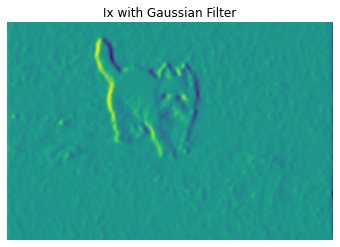
Ix_gaussian = scipy.ndimage.convolve(im_blurred_gaussian, dx, mode = "constant", cval = 0)
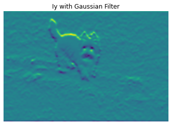
Iy_gaussian = scipy.ndimage.convolve(im_blurred_gaussian, dy, mode = "constant", cval = 0)
edges_gaussian = Ix_gaussian**2. + Iy_gaussian**2.
plt.figure()
plt.axis('off')
plt.title('Blurred Image with Gaussian Filter')
plt.imshow(im_blurred_gaussian, cmap = 'gray', vmin = 0, vmax = 1)
plt.figure()
plt.axis('off')
plt.title('Ix with Gaussian Filter')
plt.imshow(Ix_gaussian)
plt.figure()
plt.title('Iy with Gaussian Filter')
plt.axis('off')
plt.imshow(Iy_gaussian)
plt.figure()
plt.title('Edges with Gaussian Filter')
plt.axis('off')
plt.imshow(edges_gaussian, vmin = 0., vmax = np.percentile(edges_gaussian, 99))
plt.show()
### Edges with blurred image with box filter ###
print("")
print("====== Edge with blurring by box filter ======")
print("")
box_filter = make_box_filter(n = 11)
im_blurred_box = scipy.ndimage.convolve(im, box_filter, mode = "constant", cval = 0)
Ix_box = scipy.ndimage.convolve(im_blurred_box, dx, mode = "constant", cval = 0)
Iy_box = scipy.ndimage.convolve(im_blurred_box, dy, mode = "constant", cval = 0)
edges_box = Ix_box**2. + Iy_box**2.
plt.figure()
plt.axis('off')
plt.title('Blurred Image with Box Filter')
plt.imshow(im_blurred_box, cmap = 'gray', vmin = 0, vmax = 1)
plt.figure()
plt.axis('off')
plt.title('Ix with Box Filter')
plt.imshow(Ix_box)
plt.figure()
plt.title('Iy with Box Filter')
plt.axis('off')
plt.imshow(Iy_box)
plt.figure()
plt.title('Edges with Box Filter')
plt.axis('off')
plt.imshow(edges_box, vmin = 0., vmax = np.percentile(edges_box, 99))
plt.show()
######################### End solution code #########################
====== Edge without blurring ======
====== Edge with blurring by gaussian filter ======
====== Edge with blurring by box filter ======
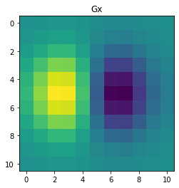
(c) Property of the convolution
Instead of convolving the image with two filters to compute $I_x$ (i.e. a Gaussian blur followed by a gradient), create a single filter $G_x$ that yields the same response. You can reuse the function in part (b). Visualize this filter using the provided code.
# Your code here!
######################### Solution code #########################
Gx = scipy.ndimage.convolve(gaussian_filter, dx, mode = "constant", cval = 0)
im_blur = scipy.ndimage.convolve(im, gaussian_filter, mode = "constant", cval = 0)
######################### End solution code #########################
plt.figure()
plt.title('Gx')
plt.imshow(Gx)
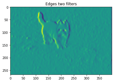
plt.figure()
plt.title('Edges two filters')
Ix = scipy.ndimage.convolve(im_blur, dx, mode = "constant", cval = 0)
plt.imshow(Ix)
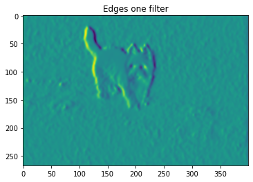
plt.figure()
plt.title('Edges one filter')
plt.imshow(scipy.ndimage.convolve(im, Gx, mode = "constant", cval = 0))
print(np.abs(np.sum(im_blur - im)))
print(np.abs(scipy.ndimage.convolve(im_blur, dx)[15:-15,15:-15] - scipy.ndimage.convolve(im, Gx)[15:-15,15:-15]).mean())
133.60071244740328
0.0018285264188413427
(d) Oriented edge detection
Good news. Petco execs are pleased with your work and have renewed our funding for several more problem sets. At our last grant meeting, however, they made an additional request. Their competitors at Petsmart have hired a team of computer vision researchers and are now computing oriented edges of their pets: rather than just estimating just the horizontal or the vertical gradients, they now provide gradients for an arbitrary angle θ. Petsmart’s method for doing this, however, is computationally expensive: they construct a new filter for each angle, and filter the image with it. Petco sees an opportunity to pull ahead of their rivals, using the class’s knowledge of steerable filters.
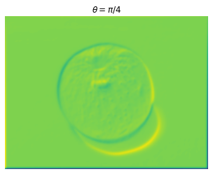
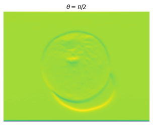
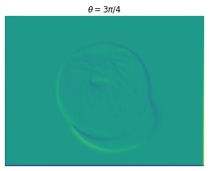
Write a function oriented_grad($I_x$, $I_y$, $\theta$) that returns the image gradient steered in the direction $\theta$, given the horizontal and vertical gradients $I_x$ and $I_y$. Use this function to compute your gradients on a blurred version of the input image at $\theta \in {\frac{1}{4}\pi, \frac{1}{2}\pi, \frac{3}{4}\pi}$, using the same Gaussian blur kernel as (b). Visualize these results in the same manner as (a).
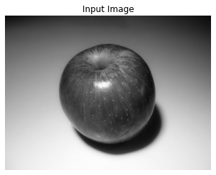
im = imageio.imread('apple.jpg').mean(2)/255.

# Your code here!
######################### Solution code #########################
def oriented_grad(Ix, Iy, theta):
  Gu = np.cos(theta) * Ix + np.sin(theta) * Iy
  return Gu

im_blurred_gaussian = scipy.ndimage.convolve(im, gaussian_filter, mode = "constant", cval = 0)
Ix = scipy.ndimage.convolve(im_blurred_gaussian, dx, mode = "constant", cval = 0)
Iy = scipy.ndimage.convolve(im_blurred_gaussian, dy, mode = "constant", cval = 0)

theta_list = [1/4 * np.pi, 1/2 * np.pi, 3/4 * np.pi]
Gu_list = [oriented_grad(Ix, Iy, theta) for theta in theta_list]
edges = [Gu ** 2 + Gu ** 2 for Gu in Gu_list]


plt.figure()
plt.axis('off')
plt.title('Input Image')
plt.imshow(im, cmap = 'gray', vmin = 0, vmax = 1)

### theta = 1/4 pi ###
plt.figure()
plt.axis('off')
plt.title(r'$\theta = \pi/4$')
plt.imshow(Gu_list[0])

### theta = 1/2 pi ###
plt.figure()
plt.axis('off')
plt.title(r'$\theta = \pi/2$')
plt.imshow(Gu_list[1])

### theta = 3/4 pi ###
plt.figure()
plt.axis('off')
plt.title(r'$\theta = 3\pi/4$')
plt.imshow(Gu_list[2])
plt.show()

######################### End solution code #########################