
HW5. Scene Recognition
Topics: MiniVGG, MiniVGG-BN, Residual Networks
import pickle
import numpy as np
import matplotlib.pyplot as plt
import os
import copy
from tqdm import tqdm

import torch
import torchvision
from torchvision import datasets, models, transforms
import torch.nn as nn
import torch.optim as optim

print("PyTorch Version: ",torch.__version__)
print("Torchvision Version: ",torchvision.__version__)
# Detect if we have a GPU available
device = torch.device("cuda:0" if torch.cuda.is_available() else "cpu")
if torch.cuda.is_available():
    print("Using the GPU!")
else:
    print("WARNING: Could not find GPU! Using CPU only. If you want to enable GPU, please to go Edit > Notebook Settings > Hardware Accelerator and select GPU.")

data_dir = "./data_miniplaces_modified"
PyTorch Version:  1.12.1+cu113
Torchvision Version:  0.13.1+cu113
Using the GPU!
Problem: Scene Recognition with VGG and ResNet
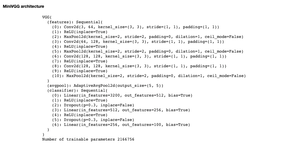
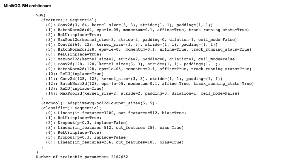
In this problem set, you will train a CNN to solve the scene recognition problem, i.e., the problem of determining which scene category a picture depicts. You will train three neural networks, which we call MiniVGG, MiniVGG-BN, and Residual Networks. MiniVGG is a smaller, simplified version of the VGG architecture, while MiniVGG-BN is identical to MiniVGG except that we added batch normalization layers after each convolution layer.
You will train the neural networks on the MiniPlaces dataset1. We’ll use 90,000 images for training, 10,000 images for validation, and the remaining 10,000 images for testing. Below is an outline for your implementation. For more detailed instructions, please refer to the notebook.
You will need to:
- Construct dataloaders for train/val/test datasets
- Build MiniVGG and MiniVGG-BN (MiniVGG with batch-normalization layers)
- Train MiniVGG and MiniVGG-BN, compare their training progresses and their final top-1 and top-5 accuracies.
- (Optional) Increase the size of the network by adding more layers and check whether top-1 and top-5 accuracies will improve.
Step 0: Downloading the dataset.
# Download the miniplaces dataset
# Note: Restarting the runtime won't remove the downloaded dataset. You only need to re-download the zip file if you lose connection to colab.
!wget http://www.eecs.umich.edu/courses/eecs504/data_miniplaces_modified.zip
--2022-10-09 17:12:08--  http://www.eecs.umich.edu/courses/eecs504/data_miniplaces_modified.zip
Resolving www.eecs.umich.edu (www.eecs.umich.edu)... 141.212.113.199
Connecting to www.eecs.umich.edu (www.eecs.umich.edu)|141.212.113.199|:80... connected.
HTTP request sent, awaiting response... 200 OK
Length: 534628730 (510M) [application/zip]
Saving to: ‘data_miniplaces_modified.zip’

data_miniplaces_mod 100%[===================>] 509.86M  1.70MB/s    in 5m 33s

2022-10-09 17:17:42 (1.53 MB/s) - ‘data_miniplaces_modified.zip’ saved [534628730/534628730]
# Unzip the download dataset .zip file to your local colab dir
# Warning: this upzipping process may take a while. Please be patient.
!unzip -q data_miniplaces_modified.zip
Step 1: Build dataloaders for train, val, and test
We often train deep neural networks on very large datasets. Because it is impossible to fit the whole dataset into the RAM, loading the data one batch at a time is a common practice. We also often need to preprocess the data, which includes common preprocessing steps like normalizing the pixel values, resizing the images to have a consistent size, and converting numpy arrays to PyTorch tensors. As the first step of this problem set, please fill in the indicated part for building data loaders with the specified data preprocessing steps (for the specific preprocessing you need to perform, please see the comments in the provided notebook). You may also find the PyTorch tutorial on data loading to be helpful.
def get_dataloaders(input_size, batch_size, shuffle = True):
    """
    Build dataloaders with transformations.

    Args:
        input_size: int, the size of the tranformed images
        batch_size: int, minibatch size for dataloading

    Returns:
        dataloader_dict: dict, dict with "train", "val", "test" keys, each is mapped to a pytorch dataloader.
    """

    mean = [0.485, 0.456, 0.406]
    std = [0.229, 0.224, 0.225]

    ###########################################################################
    # TODO: Step 1: Build transformations for the dataset.                    #
    # You need to construct a data transformation that does three             #
    # preprocessing steps in order:                                           #
    # I. Resize the image to input_size using transforms.Resize               #
    # II. Convert the image to PyTorch tensor using transforms.ToTensor       #
    # III. Normalize the images with the provided mean and std parameters     #
    # using transforms.Normalize. These parameters are accumulated from a     #
    # large number of training samples.                                       #
    # You can use transforms.Compose to combine the above three               #
    # transformations. Store the combined transforms in the variable          #
    # 'composed_transform'.                                                   #
    ###########################################################################
    composed_transform = transforms.Compose([transforms.Resize(input_size),
                                             transforms.ToTensor(),
                                             transforms.Normalize(mean, std)])
    ###########################################################################
    #                              END OF YOUR CODE                           #
    ###########################################################################

    # We write the remaining part of the dataloader for you.
    # You are encouraged to go through this.

    ###########################################################################
    # Step 2: Build dataloaders.                                              #
    # I. We use torch.datasets.ImageFolder with the provided data_dir and the #
    # data transfomations you created in step 1 to construct pytorch datasets #
    # for training, validation, and testing.                                  #
    # II. Then we use torch.utils.data.DataLoader to build dataloaders with   #
    # the constructed pytorch datasets. You need to enable shuffling for      #
    # the training set. Set num_workers=2 to speed up dataloading.            #
    # III. Finally, we put the dataloaders into a dictionary.                 #
    ###########################################################################

    # Create train/val/test datasets
    data_transforms = {
        'train': composed_transform,
        'val': composed_transform,
        'test': composed_transform
    }
    image_datasets = {x: datasets.ImageFolder(os.path.join(data_dir, x), data_transforms[x]) for x in data_transforms.keys()}

    # Create training train/val/test dataloaders
    # Never shuffle the val and test datasets
    dataloaders_dict = {x: torch.utils.data.DataLoader(image_datasets[x], batch_size=batch_size, shuffle=False if x != 'train' else shuffle, num_workers=2) for x in data_transforms.keys()}

    return dataloaders_dict
batch_size = 16
input_size = 128
dataloaders_dict = get_dataloaders(input_size, batch_size)

# Confirm your train/val/test sets contain 90,000/10,000/10,000 samples
print('# of training samples {}'.format(len(dataloaders_dict['train'].dataset)))
print('# of validation samples {}'.format(len(dataloaders_dict['val'].dataset)))
print('# of test samples {}'.format(len(dataloaders_dict['test'].dataset)))
# of training samples 90000
# of validation samples 10000
# of test samples 10000
# Visualize the data within the dataset
import json
with open('./data_miniplaces_modified/category_names.json', 'r') as f:
    class_names = json.load(f)['i2c']
class_names = {i:name for i, name in enumerate(class_names)}

def imshow(inp, title=None, ax=None, figsize=(10, 10)):
  """Imshow for Tensor."""
  inp = inp.numpy().transpose((1, 2, 0))
  mean = np.array([0.485, 0.456, 0.406])
  std = np.array([0.229, 0.224, 0.225])
  inp = std * inp + mean
  inp = np.clip(inp, 0, 1)
  if ax is None:
    fig, ax = plt.subplots(1, figsize=figsize)
  ax.imshow(inp)
  ax.set_xticks([])
  ax.set_yticks([])
  if title is not None:
    ax.set_title(title)

# Get a batch of training data
inputs, classes = next(iter(dataloaders_dict['train']))

# Make a grid from batch
out = torchvision.utils.make_grid(inputs, nrow=4)

fig, ax = plt.subplots(1, figsize=(10, 10))
title = [class_names[x.item()] if (i+1) % 4 != 0 else class_names[x.item()]+'\n' for i, x in enumerate(classes)]
imshow(out, title=' | '.join(title), ax=ax)

Step 2. Build MiniVGG and MiniVGG-BN
Construct the MiniVGG and MiniVGG-BN models. Make sure the neural networks you build have the same architectures as the ones we give in the notebook before you start training them.
# Helper function for counting number of trainable parameters.
def count_params(model):
    """
    Counts the number of trainable parameters in PyTorch.

    Args:
        model: PyTorch model.

    Returns:
        num_params: int, number of trainable parameters.
    """

    num_params = sum([item.numel() for item in model.parameters() if item.requires_grad])

    return num_params
# Network configurations for all layers before the final fully-connected layers.
# "M" corresponds to maxpooling layer, integers correspond to number of output
# channels of a convolutional layer.
cfgs = {
    'MiniVGG': [64, 'M', 128, 'M', 128, 128, 'M'],
    'MiniVGG-BN': [64, 'M', 128, 'M', 128, 128, 'M']
}

def make_layers(cfg, batch_norm=False):
    """
    Return a nn.Sequential object containing all layers to get the features
    using the CNN. (That is, before the Average pooling layer in the two
    pictures above).

    Args:
      cfg: list
      batch_norm: bool, default: False. If set to True, a BatchNorm layer
                  should be added after each convolutional layer.

    Return:
      features: torch.nn.Sequential. Containers for all feature extraction
                layers. For use of torch.nn.Sequential, please refer to
                PyTorch documentation.
    """
    ###########################################################################
    # TODO: Construct the neural net architecture from cfg. You should use    #
    # nn.Sequential().                                                        #
    ###########################################################################
    in_channel = 3
    all_layers = []
    conv_kernel_size = 3
    conv_stride = 1
    conv_padding = 1
    max_kernel_size = 2
    max_stride = 2

    for out_channel in cfg:
      if out_channel != "M":
        all_layers.append(torch.nn.Conv2d(in_channel, out_channel, kernel_size = conv_kernel_size, stride = conv_stride, padding = conv_padding))

        if batch_norm:
          all_layers.append(torch.nn.BatchNorm2d(out_channel))

        all_layers.append(torch.nn.ReLU(inplace = True))
        in_channel = out_channel

      if out_channel == "M":
        all_layers.append(torch.nn.MaxPool2d(kernel_size = max_kernel_size, stride = max_stride))

    features = torch.nn.Sequential(*all_layers)
    ###########################################################################
    #                              END OF YOUR CODE                           #
    ###########################################################################

    return features

class VGG(nn.Module):

    def __init__(self, features, num_classes=100, init_weights=True):
        super(VGG, self).__init__()

        self.features = features
        self.avgpool = nn.AdaptiveAvgPool2d((5, 5))

        #######################################################################
        # TODO: Construct the final FC layers using nn.Sequential.            #
        # Note: The average pooling layer has been defined by us above.       #
        #######################################################################
        self.classifier = torch.nn.Sequential(
                            torch.nn.Linear(3200, 512, bias = True),
                            torch.nn.ReLU(inplace = True),
                            torch.nn.Dropout(p = 0.3, inplace = False),
                            torch.nn.Linear(512, 256, bias = True),
                            torch.nn.ReLU(inplace = True),
                            torch.nn.Dropout(p = 0.3, inplace = False),
                            torch.nn.Linear(256, num_classes, bias = True)
        )
        #######################################################################
        #                              END OF YOUR CODE                       #
        #######################################################################

        if init_weights:
            self._initialize_weights()

    def forward(self, x):
        x = self.features(x)
        x = self.avgpool(x)
        x = torch.flatten(x, 1)
        x = self.classifier(x)
        return x

    def _initialize_weights(self):
        for m in self.modules():
            if isinstance(m, nn.Conv2d):
                nn.init.kaiming_normal_(m.weight, mode='fan_out', nonlinearity='relu')
                if m.bias is not None:
                    nn.init.constant_(m.bias, 0)
            elif isinstance(m, nn.BatchNorm2d):
                nn.init.constant_(m.weight, 1)
                nn.init.constant_(m.bias, 0)
            elif isinstance(m, nn.Linear):
                nn.init.normal_(m.weight, 0, 0.01)
                nn.init.constant_(m.bias, 0)
features = make_layers(cfgs['MiniVGG'], batch_norm=False)
vgg = VGG(features)

features = make_layers(cfgs['MiniVGG-BN'], batch_norm=True)
vgg_bn = VGG(features)

# Print the network architectrue. Please compare the printed architecture with
# the one given in the instructions above.
# Make sure your network has the same architecture as the one we give above.
print(vgg)
print('Number of trainable parameters {}'.format(count_params(vgg)))

print(vgg_bn)
print('Number of trainable parameters {}'.format(count_params(vgg_bn)))
VGG(
  (features): Sequential(
    (0): Conv2d(3, 64, kernel_size=(3, 3), stride=(1, 1), padding=(1, 1))
    (1): ReLU(inplace=True)
    (2): MaxPool2d(kernel_size=2, stride=2, padding=0, dilation=1, ceil_mode=False)
    (3): Conv2d(64, 128, kernel_size=(3, 3), stride=(1, 1), padding=(1, 1))
    (4): ReLU(inplace=True)
    (5): MaxPool2d(kernel_size=2, stride=2, padding=0, dilation=1, ceil_mode=False)
    (6): Conv2d(128, 128, kernel_size=(3, 3), stride=(1, 1), padding=(1, 1))
    (7): ReLU(inplace=True)
    (8): Conv2d(128, 128, kernel_size=(3, 3), stride=(1, 1), padding=(1, 1))
    (9): ReLU(inplace=True)
    (10): MaxPool2d(kernel_size=2, stride=2, padding=0, dilation=1, ceil_mode=False)
  )
  (avgpool): AdaptiveAvgPool2d(output_size=(5, 5))
  (classifier): Sequential(
    (0): Linear(in_features=3200, out_features=512, bias=True)
    (1): ReLU(inplace=True)
    (2): Dropout(p=0.3, inplace=False)
    (3): Linear(in_features=512, out_features=256, bias=True)
    (4): ReLU(inplace=True)
    (5): Dropout(p=0.3, inplace=False)
    (6): Linear(in_features=256, out_features=100, bias=True)
  )
)
Number of trainable parameters 2166756
VGG(
  (features): Sequential(
    (0): Conv2d(3, 64, kernel_size=(3, 3), stride=(1, 1), padding=(1, 1))
    (1): BatchNorm2d(64, eps=1e-05, momentum=0.1, affine=True, track_running_stats=True)
    (2): ReLU(inplace=True)
    (3): MaxPool2d(kernel_size=2, stride=2, padding=0, dilation=1, ceil_mode=False)
    (4): Conv2d(64, 128, kernel_size=(3, 3), stride=(1, 1), padding=(1, 1))
    (5): BatchNorm2d(128, eps=1e-05, momentum=0.1, affine=True, track_running_stats=True)
    (6): ReLU(inplace=True)
    (7): MaxPool2d(kernel_size=2, stride=2, padding=0, dilation=1, ceil_mode=False)
    (8): Conv2d(128, 128, kernel_size=(3, 3), stride=(1, 1), padding=(1, 1))
    (9): BatchNorm2d(128, eps=1e-05, momentum=0.1, affine=True, track_running_stats=True)
    (10): ReLU(inplace=True)
    (11): Conv2d(128, 128, kernel_size=(3, 3), stride=(1, 1), padding=(1, 1))
    (12): BatchNorm2d(128, eps=1e-05, momentum=0.1, affine=True, track_running_stats=True)
    (13): ReLU(inplace=True)
    (14): MaxPool2d(kernel_size=2, stride=2, padding=0, dilation=1, ceil_mode=False)
  )
  (avgpool): AdaptiveAvgPool2d(output_size=(5, 5))
  (classifier): Sequential(
    (0): Linear(in_features=3200, out_features=512, bias=True)
    (1): ReLU(inplace=True)
    (2): Dropout(p=0.3, inplace=False)
    (3): Linear(in_features=512, out_features=256, bias=True)
    (4): ReLU(inplace=True)
    (5): Dropout(p=0.3, inplace=False)
    (6): Linear(in_features=256, out_features=100, bias=True)
  )
)
Number of trainable parameters 2167652
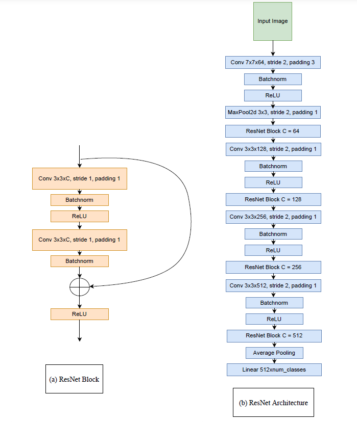
Step 3. Build small ResNet model (EECS 504)
Implement the residual block. Each block applies two convolutions and uses a residual connection. We will implement this as a class ResidualBlock, which is parameterized with the number of channels.
ResNet architecture
# For EECS 504 students only other please delete/comment this cell

class ResidualBlock(nn.Module):
    def __init__(self, in_channels, out_channels, stride = 1):
        super(ResidualBlock, self).__init__()
        ###########################################################################
        # TODO: Code the residual block as depicted in the above figure. You should use    #
        # nn.Sequential().                                                        #
        ###########################################################################
        self.inner_block = torch.nn.Sequential(
                               torch.nn.Conv2d(in_channels = in_channels, out_channels = out_channels, kernel_size = 3, stride = stride, padding = 1),
                               torch.nn.BatchNorm2d(out_channels),
                               torch.nn.ReLU(),
                               torch.nn.Conv2d(in_channels = out_channels, out_channels = in_channels, kernel_size = 3, stride = stride, padding = 1),
                               torch.nn.BatchNorm2d(in_channels)
                           )
        #######################################################################
        #                              END OF YOUR CODE                       #
        #######################################################################

    def forward(self, x):

        ###########################################################################
        # TODO: Code the forward pass for the residual block as depicted in the above figure.
        # Note: The relu activation function is after the skip connection.                                                        #
        ###########################################################################
        x = self.inner_block(x) + x
        out = torch.nn.ReLU()(x)
        #######################################################################
        #                              END OF YOUR CODE                       #
        #######################################################################
        return out
# For EECS 504 students only other please delete/comment this cell

class ResNet(nn.Module):
    def __init__(self, block, layers, num_classes = 100):
        super(ResNet, self).__init__()

        ###########################################################################
        # TODO: Construct the neural net architecture for the resnet model. You should use nn.Sequential().
        # Note: We already implemented most of the network you just need to code the initial layers and insert the residual blocks.
        ###########################################################################

        self.backbone = nn.Sequential(
                        ###########################################################################
                        # TODO: Code the initial layers i.e the the strided convolution layer, batchnorm, relu, maxpool layer and the residual blocks
                        #Hint: you have to make use of the "block" variable.
                        ###########################################################################
                        nn.Sequential(
                            nn.Conv2d(in_channels = 3, out_channels = 64, kernel_size = 7, stride = 2, padding = 3),
                            nn.BatchNorm2d(64),
                            nn.ReLU(),
                            nn.MaxPool2d(kernel_size = 3, stride = 2, padding = 1),
                            block(in_channels = 64, out_channels = 64)
                        ),
                        #######################################################################
                        #                              END OF YOUR CODE                       #
                        #######################################################################
                        nn.Sequential(
                        nn.Conv2d(64, 128, kernel_size = 3, stride = 2, padding = 1),
                        nn.BatchNorm2d(128),
                        nn.ReLU()),
                        ###########################################################################
                        # TODO: Inser the residual block please follow the figure for the number of channels and the flow of layers.
                        ###########################################################################
                        block(in_channels = 128, out_channels = 128),
                        #######################################################################
                        #                              END OF YOUR CODE                       #
                        #######################################################################
                        nn.Sequential(
                        nn.Conv2d(128, 256, kernel_size = 3, stride = 2, padding = 1),
                        nn.BatchNorm2d(256),
                        nn.ReLU()),
                        ###########################################################################
                        # TODO: Inser the residual block please follow the figure for the number of channels and the flow of layers.
                        ###########################################################################
                        block(in_channels = 256, out_channels = 256),
                        #######################################################################
                        #                              END OF YOUR CODE                       #
                        #######################################################################
                        nn.Sequential(
                        nn.Conv2d(256, 512, kernel_size = 3, stride = 2, padding = 1),
                        nn.BatchNorm2d(512),
                        nn.ReLU()),
                        ###########################################################################
                        # TODO: Inser the residual block please follow the figure for the number of channels and the flow of layers.
                        ###########################################################################
                        block(in_channels = 512, out_channels = 512)
                        #######################################################################
                        #                              END OF YOUR CODE                       #
                        #######################################################################
        )


        self.avgpool = nn.AvgPool2d(2, stride=1)
        self.fc = nn.Linear(512, num_classes)


    def forward(self, x):
        x = self.backbone(x)
        x = self.avgpool(x)
        x = x.view(x.size(0), -1)
        x = self.fc(x)

        return x
# For EECS 504 students only other please delete/comment this cell

resnet = ResNet(ResidualBlock, [1, 1, 1, 1], 100)
print(resnet)
print('Number of trainable parameters {}'.format(count_params(resnet)))
ResNet(
  (backbone): Sequential(
    (0): Sequential(
      (0): Conv2d(3, 64, kernel_size=(7, 7), stride=(2, 2), padding=(3, 3))
      (1): BatchNorm2d(64, eps=1e-05, momentum=0.1, affine=True, track_running_stats=True)
      (2): ReLU()
      (3): MaxPool2d(kernel_size=3, stride=2, padding=1, dilation=1, ceil_mode=False)
      (4): ResidualBlock(
        (inner_block): Sequential(
          (0): Conv2d(64, 64, kernel_size=(3, 3), stride=(1, 1), padding=(1, 1))
          (1): BatchNorm2d(64, eps=1e-05, momentum=0.1, affine=True, track_running_stats=True)
          (2): ReLU()
          (3): Conv2d(64, 64, kernel_size=(3, 3), stride=(1, 1), padding=(1, 1))
          (4): BatchNorm2d(64, eps=1e-05, momentum=0.1, affine=True, track_running_stats=True)
        )
      )
    )
    (1): Sequential(
      (0): Conv2d(64, 128, kernel_size=(3, 3), stride=(2, 2), padding=(1, 1))
      (1): BatchNorm2d(128, eps=1e-05, momentum=0.1, affine=True, track_running_stats=True)
      (2): ReLU()
    )
    (2): ResidualBlock(
      (inner_block): Sequential(
        (0): Conv2d(128, 128, kernel_size=(3, 3), stride=(1, 1), padding=(1, 1))
        (1): BatchNorm2d(128, eps=1e-05, momentum=0.1, affine=True, track_running_stats=True)
        (2): ReLU()
        (3): Conv2d(128, 128, kernel_size=(3, 3), stride=(1, 1), padding=(1, 1))
        (4): BatchNorm2d(128, eps=1e-05, momentum=0.1, affine=True, track_running_stats=True)
      )
    )
    (3): Sequential(
      (0): Conv2d(128, 256, kernel_size=(3, 3), stride=(2, 2), padding=(1, 1))
      (1): BatchNorm2d(256, eps=1e-05, momentum=0.1, affine=True, track_running_stats=True)
      (2): ReLU()
    )
    (4): ResidualBlock(
      (inner_block): Sequential(
        (0): Conv2d(256, 256, kernel_size=(3, 3), stride=(1, 1), padding=(1, 1))
        (1): BatchNorm2d(256, eps=1e-05, momentum=0.1, affine=True, track_running_stats=True)
        (2): ReLU()
        (3): Conv2d(256, 256, kernel_size=(3, 3), stride=(1, 1), padding=(1, 1))
        (4): BatchNorm2d(256, eps=1e-05, momentum=0.1, affine=True, track_running_stats=True)
      )
    )
    (5): Sequential(
      (0): Conv2d(256, 512, kernel_size=(3, 3), stride=(2, 2), padding=(1, 1))
      (1): BatchNorm2d(512, eps=1e-05, momentum=0.1, affine=True, track_running_stats=True)
      (2): ReLU()
    )
    (6): ResidualBlock(
      (inner_block): Sequential(
        (0): Conv2d(512, 512, kernel_size=(3, 3), stride=(1, 1), padding=(1, 1))
        (1): BatchNorm2d(512, eps=1e-05, momentum=0.1, affine=True, track_running_stats=True)
        (2): ReLU()
        (3): Conv2d(512, 512, kernel_size=(3, 3), stride=(1, 1), padding=(1, 1))
        (4): BatchNorm2d(512, eps=1e-05, momentum=0.1, affine=True, track_running_stats=True)
      )
    )
  )
  (avgpool): AvgPool2d(kernel_size=2, stride=1, padding=0)
  (fc): Linear(in_features=512, out_features=100, bias=True)
)
Number of trainable parameters 7884516
Step 4: Build training/validation loops
Implement the training and validation loops. For the training loop, you will need to implement the following steps: i) compute the outputs for each minibatch using the neural networks you build, ii) calculate the loss, iii) update the parameters using the SGD optimizer (with momentum). Please use PyTorch’s built-in automatic differentiation, rather than implementing backprogagation yourself. The validation loop is almost identical to the training loop except that we do not perform gradient update to the model parameters; we’ll simply report the loss and accuracy. Please see the notebook as well for further instructions.
def make_optimizer(model):
    """
    Args:
        model: NN to train

    Returns:
        optimizer: pytorch optmizer for updating the given model parameters.
    """
    ###########################################################################
    # TODO: Create a SGD optimizer with learning rate=1e-2 and momentum=0.9.  #
    # HINT: Check out optim.SGD() and initialize it with the appropriate      #
    # parameters. We have imported torch.optim as optim for you above.        #
    ###########################################################################
    optimizer = optim.SGD(model.parameters(), lr = 1e-2, momentum = 0.9)
    ###########################################################################
    #                              END OF YOUR CODE                           #
    ###########################################################################
    return optimizer

def get_loss():
    """
    Returns:
        criterion: pytorch loss.
    """
    ###########################################################################
    # TODO: Create an instance of the cross entropy loss. This code           #
    # should be a one-liner.                                                  #
    ###########################################################################
    criterion = torch.nn.CrossEntropyLoss()
    ###########################################################################
    #                              END OF YOUR CODE                           #
    ###########################################################################

    return criterion
def train_model(model, dataloaders, criterion, optimizer, save_dir = None, num_epochs=25, model_name='MiniVGG'):
    """
    Args:
        model: The NN to train
        dataloaders: A dictionary containing at least the keys
                    'train','val' that maps to Pytorch data loaders for the dataset
        criterion: The Loss function
        optimizer: Pytroch optimizer. The algorithm to update weights
        num_epochs: How many epochs to train for
        save_dir: Where to save the best model weights that are found. Using None will not write anything to disk.

    Returns:
        model: The trained NN
        tr_acc_history: list, training accuracy history. Recording freq: one epoch.
        val_acc_history: list, validation accuracy history. Recording freq: one epoch.
    """

    val_acc_history = []
    tr_acc_history = []

    best_model_wts = copy.deepcopy(model.state_dict())
    best_acc = 0.0

    for epoch in range(num_epochs):
        print('Epoch {}/{}'.format(epoch, num_epochs - 1))
        print('-' * 10)

        # Each epoch has a training and validation phase
        for phase in ['train', 'val']:
            if phase == 'train':
                model.train()  # Set model to training mode
            else:
                model.eval()   # Set model to evaluate mode

            # loss and number of correct prediction for the current batch
            running_loss = 0.0
            running_corrects = 0

            # Iterate over data.
            # TQDM has nice progress bars
            for inputs, labels in tqdm(dataloaders[phase]):
                inputs = inputs.to(device)
                labels = labels.to(device)

                ###############################################################
                # TODO:                                                       #
                # Please read all the inputs carefully!                       #
                # For "train" phase:                                          #
                # (i)   Compute the outputs using the model                   #
                #       Also, use the  outputs to calculate the class         #
                #       predicted by the model,                               #
                #       Store the predicted class in 'preds'                  #
                #       (Think: argmax of outputs across a dimension)         #
                #       torch.max() might help!                               #
                # (ii)  Use criterion to store the loss in 'loss'             #
                # (iii) Update the model parameters                           #
                # Notes:                                                      #
                # - Don't forget to zero the gradients before beginning the   #
                # loop!                                                       #
                # - "val" phase is the same as train, but without backprop    #
                # - Compute the outputs (Same as "train", calculate 'preds'   #
                # too),                                                       #
                # - Calculate the loss and store it in 'loss'                 #
                ###############################################################
                optimizer.zero_grad()

                outputs = model(inputs)
                preds = torch.max(outputs, 1)[1]
                loss = criterion(outputs, labels)

                if phase == "train":
                  loss.backward()
                  optimizer.step()
                ###############################################################
                #                         END OF YOUR CODE                    #
                ###############################################################

                # statistics
                running_loss += loss.item() * inputs.size(0)
                running_corrects += torch.sum(preds == labels.data)

            epoch_loss = running_loss / len(dataloaders[phase].dataset)
            epoch_acc = running_corrects.double() / len(dataloaders[phase].dataset)

            print('{} Loss: {:.4f} Acc: {:.4f}'.format(phase, epoch_loss, epoch_acc))

            # deep copy the model
            if phase == 'val' and epoch_acc > best_acc:
                best_acc = epoch_acc
                best_model_wts = copy.deepcopy(model.state_dict())

                # save the best model weights
                # =========================================================== #
                # IMPORTANT:
                # Losing your connection to colab will lead to loss of trained
                # weights.
                # You should download the trained weights to your local machine.
                # Later, you can load these weights directly without needing to
                # train the neural networks again.
                # =========================================================== #
                if save_dir:
                    torch.save(best_model_wts, os.path.join(save_dir, model_name + '.pth'))

            # record the train/val accuracies
            if phase == 'val':
                val_acc_history.append(epoch_acc)
            else:
                tr_acc_history.append(epoch_acc)

    print('Best val Acc: {:4f}'.format(best_acc))

    return model, tr_acc_history, val_acc_history
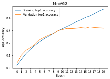
Step 5. Train MiniVGG / MiniVGG-BN and ResNet model (EECS 504)
Train the networks and visualize training and validation accuracy history for MiniVGG, MiniVGG-BN, and ResNet using the code we provide in the notebook. Comment on the effect of batch normalization. Please leave your comments in the text block we provide at the end of Step 4 section in the notebook. Note: training each neural network will take about 25 minutes.
# Number of classes in the dataset
# Miniplaces has 100
num_classes = 100

# Batch size for training
batch_size = 128

# Shuffle the input data?
shuffle_datasets = True

# Number of epochs to train for
# During debugging, you can set this parameter to 1
# num_epochs = 1
# Training for 20 epochs. This will take about half an hour.
num_epochs = 20

### IO
# Directory to save weights to
save_dir = "weights"
os.makedirs(save_dir, exist_ok=True)

# get dataloaders and criterion function
input_size = 64
dataloaders = get_dataloaders(input_size, batch_size, shuffle_datasets)
criterion = get_loss()
# Initialize MiniVGG
features = make_layers(cfgs['MiniVGG'], batch_norm=False)
model = VGG(features).to(device)
optimizer = make_optimizer(model)

# Train the model!
vgg, tr_his, val_his = train_model(model=model, dataloaders=dataloaders, criterion=criterion, optimizer=optimizer,
           save_dir=save_dir, num_epochs=num_epochs, model_name='MiniVGG')
Epoch 0/19
----------


100%|██████████| 704/704 [01:19<00:00,  8.83it/s]


train Loss: 4.5134 Acc: 0.0197


100%|██████████| 79/79 [00:07<00:00, 10.15it/s]


val Loss: 4.2325 Acc: 0.0378
Epoch 1/19
----------


100%|██████████| 704/704 [01:11<00:00,  9.84it/s]


train Loss: 4.0698 Acc: 0.0672


100%|██████████| 79/79 [00:07<00:00, 10.26it/s]


val Loss: 3.8137 Acc: 0.1021
Epoch 2/19
----------


100%|██████████| 704/704 [01:11<00:00,  9.81it/s]


train Loss: 3.7588 Acc: 0.1148


100%|██████████| 79/79 [00:07<00:00, 10.37it/s]


val Loss: 3.5763 Acc: 0.1404
Epoch 3/19
----------


100%|██████████| 704/704 [01:13<00:00,  9.64it/s]


train Loss: 3.5403 Acc: 0.1493


100%|██████████| 79/79 [00:07<00:00, 10.43it/s]


val Loss: 3.4597 Acc: 0.1625
Epoch 4/19
----------


100%|██████████| 704/704 [01:10<00:00,  9.97it/s]


train Loss: 3.3585 Acc: 0.1811


100%|██████████| 79/79 [00:07<00:00, 10.43it/s]


val Loss: 3.3164 Acc: 0.1887
Epoch 5/19
----------


100%|██████████| 704/704 [01:11<00:00,  9.88it/s]


train Loss: 3.2088 Acc: 0.2087


100%|██████████| 79/79 [00:07<00:00, 10.29it/s]


val Loss: 3.1481 Acc: 0.2262
Epoch 6/19
----------


100%|██████████| 704/704 [01:10<00:00,  9.94it/s]


train Loss: 3.0728 Acc: 0.2343


100%|██████████| 79/79 [00:07<00:00, 10.36it/s]


val Loss: 3.0075 Acc: 0.2444
Epoch 7/19
----------


100%|██████████| 704/704 [01:11<00:00,  9.91it/s]


train Loss: 2.9659 Acc: 0.2540


100%|██████████| 79/79 [00:07<00:00, 10.17it/s]


val Loss: 2.9788 Acc: 0.2625
Epoch 8/19
----------


100%|██████████| 704/704 [01:11<00:00,  9.87it/s]


train Loss: 2.8591 Acc: 0.2751


100%|██████████| 79/79 [00:07<00:00, 10.64it/s]


val Loss: 2.8858 Acc: 0.2735
Epoch 9/19
----------


100%|██████████| 704/704 [01:09<00:00, 10.14it/s]


train Loss: 2.7651 Acc: 0.2971


100%|██████████| 79/79 [00:07<00:00, 10.73it/s]


val Loss: 2.7796 Acc: 0.2983
Epoch 10/19
----------


100%|██████████| 704/704 [01:09<00:00, 10.17it/s]


train Loss: 2.6643 Acc: 0.3142


100%|██████████| 79/79 [00:07<00:00, 10.62it/s]


val Loss: 2.7357 Acc: 0.3072
Epoch 11/19
----------


100%|██████████| 704/704 [01:10<00:00,  9.98it/s]


train Loss: 2.5806 Acc: 0.3310


100%|██████████| 79/79 [00:07<00:00, 10.56it/s]


val Loss: 2.7168 Acc: 0.3158
Epoch 12/19
----------


100%|██████████| 704/704 [01:09<00:00, 10.10it/s]


train Loss: 2.4940 Acc: 0.3489


100%|██████████| 79/79 [00:07<00:00, 10.77it/s]


val Loss: 2.7142 Acc: 0.3143
Epoch 13/19
----------


100%|██████████| 704/704 [01:08<00:00, 10.25it/s]


train Loss: 2.4009 Acc: 0.3696


100%|██████████| 79/79 [00:07<00:00, 10.64it/s]


val Loss: 2.6908 Acc: 0.3171
Epoch 14/19
----------


100%|██████████| 704/704 [01:09<00:00, 10.15it/s]


train Loss: 2.3184 Acc: 0.3849


100%|██████████| 79/79 [00:07<00:00, 10.52it/s]


val Loss: 2.6728 Acc: 0.3228
Epoch 15/19
----------


100%|██████████| 704/704 [01:09<00:00, 10.08it/s]


train Loss: 2.2317 Acc: 0.4033


100%|██████████| 79/79 [00:07<00:00, 10.61it/s]


val Loss: 2.6955 Acc: 0.3179
Epoch 16/19
----------


100%|██████████| 704/704 [01:10<00:00,  9.95it/s]


train Loss: 2.1600 Acc: 0.4155


100%|██████████| 79/79 [00:07<00:00, 10.72it/s]


val Loss: 2.7149 Acc: 0.3273
Epoch 17/19
----------


100%|██████████| 704/704 [01:10<00:00, 10.03it/s]


train Loss: 2.0860 Acc: 0.4341


100%|██████████| 79/79 [00:07<00:00, 10.51it/s]


val Loss: 2.7173 Acc: 0.3231
Epoch 18/19
----------


100%|██████████| 704/704 [01:09<00:00, 10.07it/s]


train Loss: 1.9902 Acc: 0.4547


100%|██████████| 79/79 [00:07<00:00, 10.35it/s]


val Loss: 2.7501 Acc: 0.3207
Epoch 19/19
----------


100%|██████████| 704/704 [01:09<00:00, 10.16it/s]


train Loss: 1.9151 Acc: 0.4696


100%|██████████| 79/79 [00:07<00:00, 10.66it/s]

val Loss: 2.8134 Acc: 0.3176
Best val Acc: 0.327300
# Initialize MiniVGG-BN
features = make_layers(cfgs['MiniVGG-BN'], batch_norm=True)
model = VGG(features).to(device)
optimizer = make_optimizer(model)

# Train the model!
vgg_BN, tr_his_BN, val_his_BN = train_model(model=model, dataloaders=dataloaders, criterion=criterion, optimizer=optimizer,
           save_dir=save_dir, num_epochs=num_epochs, model_name='MiniVGG-BN')
Epoch 0/19
----------


100%|██████████| 704/704 [01:11<00:00,  9.79it/s]


train Loss: 4.2134 Acc: 0.0461


100%|██████████| 79/79 [00:07<00:00, 10.50it/s]


val Loss: 3.7791 Acc: 0.0974
Epoch 1/19
----------


100%|██████████| 704/704 [01:10<00:00,  9.98it/s]


train Loss: 3.6223 Acc: 0.1288


100%|██████████| 79/79 [00:07<00:00, 10.40it/s]


val Loss: 3.4260 Acc: 0.1645
Epoch 2/19
----------


100%|██████████| 704/704 [01:10<00:00,  9.93it/s]


train Loss: 3.3486 Acc: 0.1757


100%|██████████| 79/79 [00:07<00:00, 10.56it/s]


val Loss: 3.2848 Acc: 0.1814
Epoch 3/19
----------


100%|██████████| 704/704 [01:10<00:00, 10.00it/s]


train Loss: 3.1866 Acc: 0.2054


100%|██████████| 79/79 [00:07<00:00, 10.68it/s]


val Loss: 3.2472 Acc: 0.1986
Epoch 4/19
----------


100%|██████████| 704/704 [01:11<00:00,  9.87it/s]


train Loss: 3.0679 Acc: 0.2281


100%|██████████| 79/79 [00:07<00:00, 10.48it/s]


val Loss: 3.0286 Acc: 0.2367
Epoch 5/19
----------


100%|██████████| 704/704 [01:11<00:00,  9.88it/s]


train Loss: 2.9589 Acc: 0.2534


100%|██████████| 79/79 [00:07<00:00, 10.50it/s]


val Loss: 3.0092 Acc: 0.2478
Epoch 6/19
----------


100%|██████████| 704/704 [01:10<00:00,  9.95it/s]


train Loss: 2.8688 Acc: 0.2687


100%|██████████| 79/79 [00:07<00:00, 10.49it/s]


val Loss: 2.8323 Acc: 0.2738
Epoch 7/19
----------


100%|██████████| 704/704 [01:10<00:00, 10.02it/s]


train Loss: 2.7835 Acc: 0.2859


100%|██████████| 79/79 [00:07<00:00, 10.78it/s]


val Loss: 2.8044 Acc: 0.2826
Epoch 8/19
----------


100%|██████████| 704/704 [01:11<00:00,  9.89it/s]


train Loss: 2.7084 Acc: 0.3036


100%|██████████| 79/79 [00:07<00:00, 10.60it/s]


val Loss: 2.7911 Acc: 0.2854
Epoch 9/19
----------


100%|██████████| 704/704 [01:10<00:00,  9.94it/s]


train Loss: 2.6347 Acc: 0.3155


100%|██████████| 79/79 [00:07<00:00, 10.55it/s]


val Loss: 2.6828 Acc: 0.3163
Epoch 10/19
----------


100%|██████████| 704/704 [01:10<00:00,  9.99it/s]


train Loss: 2.5729 Acc: 0.3294


100%|██████████| 79/79 [00:07<00:00, 10.53it/s]


val Loss: 2.6428 Acc: 0.3197
Epoch 11/19
----------


100%|██████████| 704/704 [01:10<00:00, 10.01it/s]


train Loss: 2.5022 Acc: 0.3435


100%|██████████| 79/79 [00:07<00:00, 10.59it/s]


val Loss: 2.6157 Acc: 0.3249
Epoch 12/19
----------


100%|██████████| 704/704 [01:10<00:00,  9.92it/s]


train Loss: 2.4458 Acc: 0.3568


100%|██████████| 79/79 [00:07<00:00, 10.63it/s]


val Loss: 2.5582 Acc: 0.3427
Epoch 13/19
----------


100%|██████████| 704/704 [01:10<00:00,  9.99it/s]


train Loss: 2.3791 Acc: 0.3710


100%|██████████| 79/79 [00:07<00:00, 10.45it/s]


val Loss: 2.5809 Acc: 0.3327
Epoch 14/19
----------


100%|██████████| 704/704 [01:11<00:00,  9.85it/s]


train Loss: 2.3237 Acc: 0.3827


100%|██████████| 79/79 [00:07<00:00, 10.59it/s]


val Loss: 2.5560 Acc: 0.3428
Epoch 15/19
----------


100%|██████████| 704/704 [01:11<00:00,  9.91it/s]


train Loss: 2.2680 Acc: 0.3933


100%|██████████| 79/79 [00:07<00:00, 10.59it/s]


val Loss: 2.5894 Acc: 0.3384
Epoch 16/19
----------


100%|██████████| 704/704 [01:11<00:00,  9.91it/s]


train Loss: 2.2103 Acc: 0.4049


100%|██████████| 79/79 [00:07<00:00, 10.64it/s]


val Loss: 2.6039 Acc: 0.3380
Epoch 17/19
----------


100%|██████████| 704/704 [01:11<00:00,  9.86it/s]


train Loss: 2.1577 Acc: 0.4157


100%|██████████| 79/79 [00:07<00:00, 10.20it/s]


val Loss: 2.5385 Acc: 0.3499
Epoch 18/19
----------


100%|██████████| 704/704 [01:11<00:00,  9.90it/s]


train Loss: 2.0942 Acc: 0.4318


100%|██████████| 79/79 [00:07<00:00, 10.42it/s]


val Loss: 2.4937 Acc: 0.3603
Epoch 19/19
----------


100%|██████████| 704/704 [01:10<00:00,  9.92it/s]


train Loss: 2.0450 Acc: 0.4394


100%|██████████| 79/79 [00:07<00:00, 10.64it/s]

val Loss: 2.5733 Acc: 0.3510
Best val Acc: 0.360300
# For EECS 504 students only other please delete/comment this cell

# Initialize ResNet
resnet = ResNet(ResidualBlock, [1, 1, 1, 1], num_classes).to(device)
optimizer = make_optimizer(resnet)

# Train the model!
resnet, tr_his_res, val_his_res = train_model(model=resnet, dataloaders=dataloaders, criterion=criterion, optimizer=optimizer,
           save_dir=save_dir, num_epochs=num_epochs, model_name='ResNet')
Epoch 0/19
----------


100%|██████████| 704/704 [01:11<00:00,  9.89it/s]


train Loss: 3.6612 Acc: 0.1357


100%|██████████| 79/79 [00:07<00:00, 10.69it/s]


val Loss: 3.4342 Acc: 0.1671
Epoch 1/19
----------


100%|██████████| 704/704 [01:11<00:00,  9.89it/s]


train Loss: 3.1298 Acc: 0.2245


100%|██████████| 79/79 [00:07<00:00, 10.56it/s]


val Loss: 3.2547 Acc: 0.2188
Epoch 2/19
----------


100%|██████████| 704/704 [01:11<00:00,  9.90it/s]


train Loss: 2.8578 Acc: 0.2775


100%|██████████| 79/79 [00:07<00:00, 10.45it/s]


val Loss: 2.9675 Acc: 0.2534
Epoch 3/19
----------


100%|██████████| 704/704 [01:11<00:00,  9.79it/s]


train Loss: 2.6299 Acc: 0.3227


100%|██████████| 79/79 [00:07<00:00, 10.61it/s]


val Loss: 2.9348 Acc: 0.2737
Epoch 4/19
----------


100%|██████████| 704/704 [01:10<00:00,  9.92it/s]


train Loss: 2.4201 Acc: 0.3658


100%|██████████| 79/79 [00:07<00:00, 10.43it/s]


val Loss: 2.8482 Acc: 0.2912
Epoch 5/19
----------


100%|██████████| 704/704 [01:11<00:00,  9.84it/s]


train Loss: 2.2049 Acc: 0.4105


100%|██████████| 79/79 [00:07<00:00, 10.58it/s]


val Loss: 2.8616 Acc: 0.2993
Epoch 6/19
----------


100%|██████████| 704/704 [01:11<00:00,  9.83it/s]


train Loss: 1.9699 Acc: 0.4646


100%|██████████| 79/79 [00:07<00:00, 10.43it/s]


val Loss: 2.9318 Acc: 0.2953
Epoch 7/19
----------


100%|██████████| 704/704 [01:11<00:00,  9.90it/s]


train Loss: 1.7117 Acc: 0.5223


100%|██████████| 79/79 [00:07<00:00, 10.61it/s]


val Loss: 3.1280 Acc: 0.2910
Epoch 8/19
----------


100%|██████████| 704/704 [01:10<00:00,  9.92it/s]


train Loss: 1.4174 Acc: 0.5954


100%|██████████| 79/79 [00:07<00:00, 10.50it/s]


val Loss: 3.3771 Acc: 0.2683
Epoch 9/19
----------


100%|██████████| 704/704 [01:11<00:00,  9.86it/s]


train Loss: 1.0944 Acc: 0.6817


100%|██████████| 79/79 [00:07<00:00, 10.62it/s]


val Loss: 3.6251 Acc: 0.2702
Epoch 10/19
----------


100%|██████████| 704/704 [01:11<00:00,  9.88it/s]


train Loss: 0.8178 Acc: 0.7555


100%|██████████| 79/79 [00:07<00:00, 10.70it/s]


val Loss: 3.9328 Acc: 0.2599
Epoch 11/19
----------


100%|██████████| 704/704 [01:11<00:00,  9.80it/s]


train Loss: 0.5260 Acc: 0.8427


100%|██████████| 79/79 [00:07<00:00, 10.22it/s]


val Loss: 4.0932 Acc: 0.2767
Epoch 12/19
----------


100%|██████████| 704/704 [01:12<00:00,  9.74it/s]


train Loss: 0.3035 Acc: 0.9137


100%|██████████| 79/79 [00:07<00:00, 10.39it/s]


val Loss: 4.4584 Acc: 0.2635
Epoch 13/19
----------


100%|██████████| 704/704 [01:12<00:00,  9.75it/s]


train Loss: 0.1601 Acc: 0.9586


100%|██████████| 79/79 [00:07<00:00, 10.34it/s]


val Loss: 4.5404 Acc: 0.2743
Epoch 14/19
----------


100%|██████████| 704/704 [01:11<00:00,  9.79it/s]


train Loss: 0.0981 Acc: 0.9768


100%|██████████| 79/79 [00:07<00:00, 10.37it/s]


val Loss: 4.6103 Acc: 0.2800
Epoch 15/19
----------


100%|██████████| 704/704 [01:11<00:00,  9.86it/s]


train Loss: 0.0428 Acc: 0.9927


100%|██████████| 79/79 [00:07<00:00, 10.55it/s]


val Loss: 4.6714 Acc: 0.2913
Epoch 16/19
----------


100%|██████████| 704/704 [01:12<00:00,  9.73it/s]


train Loss: 0.0158 Acc: 0.9984


100%|██████████| 79/79 [00:07<00:00, 10.35it/s]


val Loss: 4.6710 Acc: 0.2913
Epoch 17/19
----------


100%|██████████| 704/704 [01:11<00:00,  9.78it/s]


train Loss: 0.0067 Acc: 0.9996


100%|██████████| 79/79 [00:07<00:00, 10.45it/s]


val Loss: 4.6702 Acc: 0.2998
Epoch 18/19
----------


100%|██████████| 704/704 [01:11<00:00,  9.84it/s]


train Loss: 0.0047 Acc: 0.9997


100%|██████████| 79/79 [00:07<00:00, 10.42it/s]


val Loss: 4.7119 Acc: 0.2997
Epoch 19/19
----------


100%|██████████| 704/704 [01:11<00:00,  9.81it/s]


train Loss: 0.0034 Acc: 0.9997


100%|██████████| 79/79 [00:07<00:00, 10.57it/s]

val Loss: 4.7181 Acc: 0.2989
Best val Acc: 0.299800
x = np.arange(num_epochs)
# train/val accuracies for MiniVGG
plt.figure()
plt.plot(x, torch.tensor(tr_his, device = 'cpu'))
plt.plot(x, torch.tensor(val_his, device = 'cpu'))
plt.legend(['Training top1 accuracy', 'Validation top1 accuracy'])
plt.xticks(x)
plt.xlabel('Epoch')
plt.ylabel('Top1 Accuracy')
plt.title('MiniVGG')
plt.show()
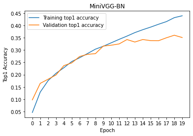
# train/val accuracies for MiniVGG-BN
plt.plot(x, torch.tensor(tr_his_BN, device = 'cpu'))
plt.plot(x, torch.tensor(val_his_BN, device = 'cpu'))
plt.legend(['Training top1 accuracy', 'Validation top1 accuracy'])
plt.xticks(x)
plt.xlabel('Epoch')
plt.ylabel('Top1 Accuracy')
plt.title('MiniVGG-BN')
plt.show()
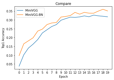
# compare val accuracies of MiniVGG and MiniVGG-BN
plt.plot(x, torch.tensor(val_his, device = 'cpu'))
plt.plot(x, torch.tensor(val_his_BN, device = 'cpu'))
plt.legend(['MiniVGG', 'MiniVGG-BN'])
plt.xticks(x)
plt.xlabel('Epoch')
plt.ylabel('Top1 Accuracy')
plt.title('Compare')
plt.show()
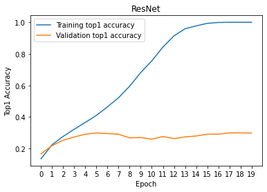
# For EECS 504 students only other please delete/comment this cell

# train/val accuracies for ResNet
plt.figure()
plt.plot(x, torch.tensor(tr_his_res, device = 'cpu'))
plt.plot(x, torch.tensor(val_his_res, device = 'cpu'))
plt.legend(['Training top1 accuracy', 'Validation top1 accuracy'])
plt.xticks(x)
plt.xlabel('Epoch')
plt.ylabel('Top1 Accuracy')
plt.title('ResNet')
plt.show()
TODO: __Summarize the effect of batch normalization:
The difference of training accuracy and validation accuracy is much smaller when we have batch normalization. So, VGG with batch normalization has higher validation accuracy than VGG without batch normalization, even if training accuracies are very similar between VGG and VGG with batch normalization.
pickle.dump(tr_his, open('tr_his.pkl', 'wb'))
pickle.dump(tr_his_BN, open('tr_his_BN.pkl', 'wb'))
pickle.dump(val_his, open('val_his.pkl', 'wb'))
pickle.dump(val_his_BN, open('val_his_BN.pkl', 'wb'))
pickle.dump(tr_his_res, open('tr_his_res.pkl', 'wb'))
pickle.dump(val_his_res, open('val_his_res.pkl', 'wb'))
Step 6. Measure top1 and top5 accuracies of MiniVGG and MiniVGG-BN
Definition of top-k accuracy: if the correct label is within the top k predicted classes according to the network output scores, we count the prediction by the neural network as a correct prediction.
If the correct label is within the top k predicted classes according to the network output scores, we count the prediction by the neural network as a correct prediction. Measure Top-1 and Top-5 accuracy on the test set (i.e. the probability that the true class appears as the most likely class, and within the Top-5 most likely respectively). To pass the test, all neural networks should have Top-5 accuracy above 55%.
def accuracy(output, target, topk=(1,)):
    """
    Computes the accuracy over the k top predictions for the specified values
    of k.

    Args:
        output: pytorch tensor, (batch_size x num_classes). Outputs of the
                network for one batch.
        target: pytorch tensor, (batch_size,). True labels for one batch.

    Returns:
        res: list. Accuracies corresponding to topk[0], topk[1], ...
    """
    with torch.no_grad():
        maxk = max(topk)
        batch_size = target.size(0)

        _, pred = output.topk(maxk, 1, True, True)
        pred = pred.t()
        correct = pred.eq(target.view(1, -1).expand_as(pred))

        res = []
        for k in topk:
            correct_k = correct[:k].reshape(-1).float().sum(0, keepdim=True)
            res.append(correct_k.mul_(100.0 / batch_size))
        return res

def test(model, dataloader):

    model.eval()

    top1_acc = []
    top5_acc = []

    with torch.no_grad():
        for inputs, labels in dataloader:
            inputs = inputs.to(device)
            labels = labels.to(device)

            outputs = model(inputs)

            res = accuracy(outputs, labels, topk=(1, 5))

            top1_acc.append(res[0] * len(outputs))
            top5_acc.append(res[1] * len(outputs))

    print('Top-1 accuracy {}%, Top-5 accuracy {}%'.format(sum(top1_acc).item()/10000, sum(top5_acc).item()/10000))
##### To pass the test, both networks should have Top-5 accuracy above 55% #####
vgg_BN.load_state_dict(torch.load('./weights/MiniVGG-BN.pth'))
vgg.load_state_dict(torch.load('./weights/MiniVGG.pth'))

test(vgg_BN, dataloaders['test'])
test(vgg, dataloaders['test'])
Top-1 accuracy 36.21%, Top-5 accuracy 66.59%
Top-1 accuracy 33.27%, Top-5 accuracy 62.29%
##### To pass the test, both networks should have Top-5 accuracy above 55% #####

# For EECS 504 students only other please delete/comment this cell

resnet.load_state_dict(torch.load('./weights/ResNet.pth'))
test(resnet, dataloaders['test'])
Top-1 accuracy 29.8%, Top-5 accuracy 57.09%