
HW6. Image Synthesis
Topics: pix2pix, conditional GAN, U-net, receptive field, style transfer
!pip install torchsummary
import pickle
import numpy as np
import matplotlib.pyplot as plt
import os
import time
import itertools
from matplotlib import image
import glob as glob
from PIL import Image

import torch
import torchvision
from torchvision import datasets, models, transforms
import torch.nn as nn
import torch.optim as optim
from torch.autograd import Variable
import torch.nn.functional as F
from torch.utils.data import DataLoader, Dataset
from torchsummary import summary

print("PyTorch Version: ",torch.__version__)
print("Torchvision Version: ",torchvision.__version__)
# Detect if we have a GPU available
device = torch.device("cuda:0" if torch.cuda.is_available() else "cpu")
if torch.cuda.is_available():
  print("Using the GPU!")
else:
  print("WARNING: Could not find GPU! Using CPU only. If you want to enable GPU, please to go Edit > Notebook Settings > Hardware Accelerator and select GPU.")
Looking in indexes: https://pypi.org/simple, https://us-python.pkg.dev/colab-wheels/public/simple/
Requirement already satisfied: torchsummary in /usr/local/lib/python3.7/dist-packages (1.5.1)
PyTorch Version:  1.12.1+cu113
Torchvision Version:  0.13.1+cu113
Using the GPU!
Problem 1. Implement pix2pix
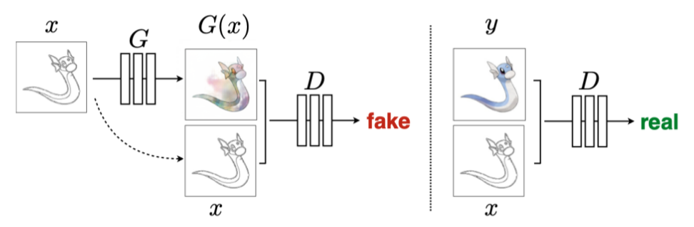
In this problem set, we will implement an image-to-image translation program based on pix2pix. We will train the pix2pix model on the edges2shoes dataset to translate images containing only the edges of a shoe, to a full image of a shoe. The edges are automatically extracted from the real shoe images.
The pix2pix model is based on a conditional GAN. The generator G maps the source image x to a synthesized target image. The discriminator takes both the source image and predicted target image as its inputs, and predicts whether the input is real or fake.
In this question, you will need to:
- Contruct dataloaders for train/test datasets
- Build Generator and Discriminator
- Train pix2pix and visualize the results during training
- Plot the loss of generator/discriminator v.s. iteration
- Design your own shoes (optional)
Step 0: Downloading the dataset.
We first download the mini-edges2shoes dataset sampled from the original edges2shoes dataset. The mini-edges2shoes dataset contains 1,000 training image pairs, and 100 testing image pairs.
There’s nothing you need to implement for this part.
# Download the mini-edges2shoes dataset
!rm -r mini-edges2shoes.zip
!rm -r mini-edges2shoes
!wget http://www.eecs.umich.edu/courses/eecs442-ahowens/mini-edges2shoes.zip
!unzip -q mini-edges2shoes.zip
rm: cannot remove 'mini-edges2shoes.zip': No such file or directory
rm: cannot remove 'mini-edges2shoes': No such file or directory
URL transformed to HTTPS due to an HSTS policy
--2022-10-27 16:51:01--  https://www.eecs.umich.edu/courses/eecs442-ahowens/mini-edges2shoes.zip
Resolving www.eecs.umich.edu (www.eecs.umich.edu)... 141.212.113.199
Connecting to www.eecs.umich.edu (www.eecs.umich.edu)|141.212.113.199|:443... connected.
HTTP request sent, awaiting response... 200 OK
Length: 48660290 (46M) [application/zip]
Saving to: ‘mini-edges2shoes.zip’

mini-edges2shoes.zi 100%[===================>]  46.41M  9.27MB/s    in 6.8s

2022-10-27 16:51:09 (6.85 MB/s) - ‘mini-edges2shoes.zip’ saved [48660290/48660290]
Step 1: Build dataloaders for train and test
We will first build data loaders for training and testing. For the training process, we will use a batch size of 4. During testing, we will process 5 images in a single batch, so that we can visualize several results at once. Please complete the Edges2Image class and fill in the TODOs in that cell.
class Edges2Image(Dataset):
  def __init__(self, root_dir, split='train', transform=None):
    """
    Args:
        root_dir: the directory of the dataset
        split: "train" or "val"
        transform: pytorch transformations.
    """

    self.transform = transform
    ###########################################################################
    # TODO: get the the file path to all train/val images                     #
    # Hint: the function glob.glob is useful                                  #
    ###########################################################################
    data_dir = root_dir + "/" + split
    self.files = glob.glob(f"{data_dir}/*.jpg")

    ###########################################################################
    #                              END OF YOUR CODE                           #
    ###########################################################################

  def __len__(self):
    return len(self.files)

  def __getitem__(self, idx):
    img = Image.open(self.files[idx])
    img = np.asarray(img)
    if self.transform:
        img = self.transform(img)
    return img

transform = transforms.Compose([
        transforms.ToTensor(),
        transforms.Normalize(mean=(0.5, 0.5, 0.5), std=(0.5, 0.5, 0.5))
])

###########################################################################
# TODO: Construct the dataloader                                          #
# For the train_loader, please use a batch size of 4 and set shuffle True #
# For the val_loader, please use a batch size of 5 and set shuffle False  #
# Hint: You'll need to create instances of the class above, name them as  #
# tr_dt and te_dt. The dataloaders should ve named as train_loader and    #
# test_loader. You also need to include transform in your class           #
#instances                                                                #
###########################################################################
ROOT_DIR = "./mini-edges2shoes"
TRAIN_BATCH_SIZE = 4
VAL_BATCH_SIZE = 5

tr_dt = Edges2Image(ROOT_DIR, "train", transform)
train_loader = DataLoader(
    tr_dt,
    batch_size = TRAIN_BATCH_SIZE,
    shuffle = True
)

te_dt = Edges2Image(ROOT_DIR, "val", transform)
test_loader = DataLoader(
    te_dt,
    batch_size = VAL_BATCH_SIZE,
    shuffle = False
)

###########################################################################
#                              END OF YOUR CODE                           #
###########################################################################

# Make sure that you have 1,000 training images and 100 testing images before moving on
print('Number of training images {}, number of testing images {}'.format(len(tr_dt), len(te_dt)))
Number of training images 1000, number of testing images 100
#Sample Output used for visualization
test = test_loader.__iter__().__next__()
img_size = 256
fixed_y_ = test[:, :, :, img_size:].cuda()
fixed_x_ = test[:, :, :, 0:img_size].cuda()
print(len(train_loader))
print(len(test_loader))
print(fixed_y_.shape)
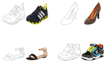
# plot sample image
fig, axes = plt.subplots(2, 2)
axes = np.reshape(axes, (4, ))
for i in range(4):
example = train_loader.__iter__().__next__()[i].numpy().transpose((1, 2, 0))
mean = np.array([0.5, 0.5, 0.5])
std = np.array([0.5, 0.5, 0.5])
example = std * example + mean
axes[i].imshow(example)
axes[i].axis('off')
plt.show()
250
20
torch.Size([5, 3, 256, 256])
Step 2: Build Generator and Discriminator
Based on the paper, the architectures of network are as following:
Generator architectures:
U-net encoder:
C64-C128-C256-C512-C512-C512-C512-C512
U-net decoder:
C512-C512-C512-C512-C256-C128-C64-C3
After the last layer in the decoder, a convolution is applied to map to the number of output channels, followed by a Tanh function. As an exception to the above notation, BatchNorm is not applied to the first C64 layer in the encoder. All ReLUs in the encoder are leaky, with slope 0.2, while ReLUs in the decoder are not leaky.
Discriminator architectures
The discriminator architecture is:
C64-C128-C256-C512
After the last layer, a convolution is applied to map to a 1-dimensional output, followed by a Sigmoid function. As an exception to the above notation, BatchNorm is not applied to the first C64 layer. All ReLUs are leaky, with slope 0.2.
We have included a toy example of a U-net architecture below. Encoder: C64-C128-C256 Decoder: C128-C64-C3
# (Not a part of your solution) Toy example of an U-net architecture
class toy_unet(nn.Module):
  # initializers
  def __init__(self):
    super(generator, self).__init__()
    # encoder
    self.conv1 = nn.Conv2d(3, 64, 4, 2, 1)
    self.conv2 = nn.Conv2d(64, 64 * 2, 4, 2, 1)
    self.conv3 = nn.Conv2d(64 * 2, 64 * 4, 4, 2, 1)
    # decoder
    self.deconv1 = nn.ConvTranspose2d(64 * 4, 64 * 2, 4, 2, 1)
    self.deconv2 = nn.ConvTranspose2d(64 * 2 * 2, 64, 4, 2, 1)
    self.deconv3 = nn.ConvTranspose2d(64 * 2, 3, 4, 2, 1)

  # forward method
  def forward(self, input):
    # pass through encoder
    e1 = self.conv1(input)
    e2 = self.conv2(F.relu(e1))
    e3 = self.conv3(F.relu(e2))
    # pass through decoder
    d1 = self.deconv1(F.relu(e3))
    d1 = torch.cat([d1, e2], 1) # Concatenation
    d2 = self.deconv2(F.relu(d1))
    d2 = torch.cat([d2, e1], 1) # Concatenation
    d3 = self.deconv3(F.relu(d2))
    return d3
def normal_init(m, mean, std):
  """
  Helper function. Initialize model parameter with given mean and std.
  """
  if isinstance(m, nn.ConvTranspose2d) or isinstance(m, nn.Conv2d):
    # delete start
    m.weight.data.normal_(mean, std)
    m.bias.data.zero_()
    # delete end
class generator(nn.Module):
  # initializers
  def __init__(self):
    super(generator, self).__init__()
    ###########################################################################
    # TODO: Build your Unet generator encoder with the layer sizes            #
    # You can also check the size with the model summary below                #
    ###########################################################################

    # C64
    self.conv1 = nn.Sequential(
      nn.Conv2d(in_channels = 3, out_channels = 64, kernel_size = 4, stride = 2, padding = 1)
    )

    # C128
    self.conv2 = nn.Sequential(
      nn.Conv2d(in_channels = 64, out_channels = 64 * 2, kernel_size = 4, stride = 2, padding = 1),
      nn.BatchNorm2d(64 * 2)
    )

    # C256
    self.conv3 = nn.Sequential(
      nn.Conv2d(in_channels = 64 * 2, out_channels = 64 * 4, kernel_size = 4, stride = 2, padding = 1),
      nn.BatchNorm2d(64 * 4)
    )

    # C512
    self.conv4 = nn.Sequential(
      nn.Conv2d(in_channels = 64 * 4, out_channels = 64 * 8, kernel_size = 4, stride = 2, padding = 1),
      nn.BatchNorm2d(64 * 8)
    )

    # C512
    self.conv5 = nn.Sequential(
      nn.Conv2d(in_channels = 64 * 8, out_channels = 64 * 8, kernel_size = 4, stride = 2, padding = 1),
      nn.BatchNorm2d(64 * 8)
    )

    # C512
    self.conv6 = nn.Sequential(
      nn.Conv2d(in_channels = 64 * 8, out_channels = 64 * 8, kernel_size = 4, stride = 2, padding = 1),
      nn.BatchNorm2d(64 * 8)
    )

    # C512
    self.conv7 = nn.Sequential(
      nn.Conv2d(in_channels = 64 * 8, out_channels = 64 * 8, kernel_size = 4, stride = 2, padding = 1),
      nn.BatchNorm2d(64 * 8)
    )

    # C512
    self.conv8 = nn.Sequential(
      nn.Conv2d(in_channels = 64 * 8, out_channels = 64 * 8, kernel_size = 4, stride = 2, padding = 1)
    )

    ###########################################################################
    #                              END OF YOUR CODE                           #
    ###########################################################################

    ###########################################################################
    # TODO: Build your Unet generator decoder with the layer sizes            #
    ###########################################################################

    # C512
    self.deconv1 = nn.Sequential(
      nn.ConvTranspose2d(in_channels = 64 * 8, out_channels = 64 * 8, kernel_size = 4, stride = 2, padding = 1),
      nn.BatchNorm2d(64 * 8)
    )

    # C512
    self.deconv2 = nn.Sequential(
      nn.ConvTranspose2d(in_channels = 64 * 8 * 2, out_channels = 64 * 8, kernel_size = 4, stride = 2, padding = 1),
      nn.BatchNorm2d(64 * 8)
    )

    # C512
    self.deconv3 = nn.Sequential(
      nn.ConvTranspose2d(in_channels = 64 * 8 * 2, out_channels = 64 * 8, kernel_size = 4, stride = 2, padding = 1),
      nn.BatchNorm2d(64 * 8)
    )

    # C512
    self.deconv4 = nn.Sequential(
      nn.ConvTranspose2d(in_channels = 64 * 8 * 2, out_channels = 64 * 8, kernel_size = 4, stride = 2, padding = 1),
      nn.BatchNorm2d(64 * 8)
    )

    # C256
    self.deconv5 = nn.Sequential(
      nn.ConvTranspose2d(in_channels = 64 * 8 * 2, out_channels = 64 * 4, kernel_size = 4, stride = 2, padding = 1),
      nn.BatchNorm2d(64 * 4)
    )

    # C128
    self.deconv6 = nn.Sequential(
      nn.ConvTranspose2d(in_channels = 64 * 4 * 2, out_channels = 64 * 2, kernel_size = 4, stride = 2, padding = 1),
      nn.BatchNorm2d(64 * 2)
    )

    # C64
    self.deconv7 = nn.Sequential(
      nn.ConvTranspose2d(in_channels = 64 * 2 * 2, out_channels = 64, kernel_size = 4, stride = 2, padding = 1),
      nn.BatchNorm2d(64)
    )

    # C3
    self.deconv8 = nn.Sequential(
      nn.ConvTranspose2d(in_channels = 64 * 2, out_channels = 3, kernel_size = 4, stride = 2, padding = 1)
    )


    ###########################################################################
    #                              END OF YOUR CODE                           #
    ###########################################################################

  # weight_init
  def weight_init(self, mean, std):
    for m in self._modules:
      normal_init(self._modules[m], mean, std)

  # forward method
  def forward(self, input):
    ###########################################################################
    # TODO: Implement the forward pass of generator                           #
    ###########################################################################
    # encoding

    e1 = F.leaky_relu(self.conv1(input), negative_slope = 0.2)
    e2 = F.leaky_relu(self.conv2(e1), negative_slope = 0.2)
    e3 = F.leaky_relu(self.conv3(e2), negative_slope = 0.2)
    e4 = F.leaky_relu(self.conv4(e3), negative_slope = 0.2)
    e5 = F.leaky_relu(self.conv5(e4), negative_slope = 0.2)
    e6 = F.leaky_relu(self.conv6(e5), negative_slope = 0.2)
    e7 = F.leaky_relu(self.conv7(e6), negative_slope = 0.2)
    e8 = F.leaky_relu(self.conv8(e7), negative_slope = 0.2)

    # decoding
    # Hint: you can use torch.cat to concatenate the decoder and the encoder inputs

    d1 = F.relu(torch.cat([self.deconv1(e8), e7] , 1))
    d2 = F.relu(torch.cat([self.deconv2(d1), e6] , 1))
    d3 = F.relu(torch.cat([self.deconv3(d2), e5] , 1))
    d4 = F.relu(torch.cat([self.deconv4(d3), e4] , 1))
    d5 = F.relu(torch.cat([self.deconv5(d4), e3] , 1))
    d6 = F.relu(torch.cat([self.deconv6(d5), e2] , 1))
    d7 = F.relu(torch.cat([self.deconv7(d6), e1] , 1))
    output = F.tanh(self.deconv8(d7))

    ###########################################################################
    #                              END OF YOUR CODE                           #
    ###########################################################################

    return output

class discriminator(nn.Module):
  # initializers
  def __init__(self):
    super(discriminator, self).__init__()
    ###########################################################################
    # TODO: Build your CNN discriminator with the layer sizes                 #
    ###########################################################################

    # C64
    self.conv1 = nn.Sequential(
        nn.Conv2d(in_channels = 3 * 2, out_channels = 64, kernel_size = 4, stride = 2, padding = 1)
    )

    # C128
    self.conv2 = nn.Sequential(
        nn.Conv2d(in_channels = 64, out_channels = 64 * 2, kernel_size = 4, stride = 2, padding = 1),
        nn.BatchNorm2d(64 * 2)
    )

    # C256
    self.conv3 = nn.Sequential(
        nn.Conv2d(in_channels = 64 * 2, out_channels = 64 * 4, kernel_size = 4, stride = 2, padding = 1),
        nn.BatchNorm2d(64 * 4)
    )

    # C512
    self.conv4 = nn.Sequential(
        nn.Conv2d(in_channels = 64 * 4, out_channels = 64 * 8, kernel_size = 4, stride = 1, padding = 1),
        nn.BatchNorm2d(64 * 8)
    )

    self.conv5 = nn.Sequential(
        nn.Conv2d(in_channels = 64 * 8, out_channels = 1, kernel_size = 4, stride = 1, padding = 1)
    )


    ###########################################################################
    #                              END OF YOUR CODE                           #
    ###########################################################################

  # weight_init
  def weight_init(self, mean, std):
    for m in self._modules:
      normal_init(self._modules[m], mean, std)

  # forward method
  def forward(self, input):
    ###########################################################################
    # TODO: Implement the forward pass of discriminator                       #
    ###########################################################################

    x = F.leaky_relu(self.conv1(input), negative_slope = 0.2)
    x = F.leaky_relu(self.conv2(x), negative_slope = 0.2)
    x = F.leaky_relu(self.conv3(x), negative_slope = 0.2)
    x = F.leaky_relu(self.conv4(x), negative_slope = 0.2)
    x = F.sigmoid(self.conv5(x))

    ###########################################################################
    #                              END OF YOUR CODE                           #
    ###########################################################################

    return x
# print out the model summary
G = generator().cuda()
D = discriminator().cuda()
summary(G, (3, 256, 256))
summary(D, (6, 256, 256))
----------------------------------------------------------------
        Layer (type)               Output Shape         Param #
================================================================
            Conv2d-1         [-1, 64, 128, 128]           3,136
            Conv2d-2          [-1, 128, 64, 64]         131,200
       BatchNorm2d-3          [-1, 128, 64, 64]             256
            Conv2d-4          [-1, 256, 32, 32]         524,544
       BatchNorm2d-5          [-1, 256, 32, 32]             512
            Conv2d-6          [-1, 512, 16, 16]       2,097,664
       BatchNorm2d-7          [-1, 512, 16, 16]           1,024
            Conv2d-8            [-1, 512, 8, 8]       4,194,816
       BatchNorm2d-9            [-1, 512, 8, 8]           1,024
           Conv2d-10            [-1, 512, 4, 4]       4,194,816
      BatchNorm2d-11            [-1, 512, 4, 4]           1,024
           Conv2d-12            [-1, 512, 2, 2]       4,194,816
      BatchNorm2d-13            [-1, 512, 2, 2]           1,024
           Conv2d-14            [-1, 512, 1, 1]       4,194,816
  ConvTranspose2d-15            [-1, 512, 2, 2]       4,194,816
      BatchNorm2d-16            [-1, 512, 2, 2]           1,024
  ConvTranspose2d-17            [-1, 512, 4, 4]       8,389,120
      BatchNorm2d-18            [-1, 512, 4, 4]           1,024
  ConvTranspose2d-19            [-1, 512, 8, 8]       8,389,120
      BatchNorm2d-20            [-1, 512, 8, 8]           1,024
  ConvTranspose2d-21          [-1, 512, 16, 16]       8,389,120
      BatchNorm2d-22          [-1, 512, 16, 16]           1,024
  ConvTranspose2d-23          [-1, 256, 32, 32]       4,194,560
      BatchNorm2d-24          [-1, 256, 32, 32]             512
  ConvTranspose2d-25          [-1, 128, 64, 64]       1,048,704
      BatchNorm2d-26          [-1, 128, 64, 64]             256
  ConvTranspose2d-27         [-1, 64, 128, 128]         262,208
      BatchNorm2d-28         [-1, 64, 128, 128]             128
  ConvTranspose2d-29          [-1, 3, 256, 256]           6,147
================================================================
Total params: 54,419,459
Trainable params: 54,419,459
Non-trainable params: 0
----------------------------------------------------------------
Input size (MB): 0.75
Forward/backward pass size (MB): 54.82
Params size (MB): 207.59
Estimated Total Size (MB): 263.16
----------------------------------------------------------------
----------------------------------------------------------------
        Layer (type)               Output Shape         Param #
================================================================
            Conv2d-1         [-1, 64, 128, 128]           6,208
            Conv2d-2          [-1, 128, 64, 64]         131,200
       BatchNorm2d-3          [-1, 128, 64, 64]             256
            Conv2d-4          [-1, 256, 32, 32]         524,544
       BatchNorm2d-5          [-1, 256, 32, 32]             512
            Conv2d-6          [-1, 512, 31, 31]       2,097,664
       BatchNorm2d-7          [-1, 512, 31, 31]           1,024
            Conv2d-8            [-1, 1, 30, 30]           8,193
================================================================
Total params: 2,769,601
Trainable params: 2,769,601
Non-trainable params: 0
----------------------------------------------------------------
Input size (MB): 1.50
Forward/backward pass size (MB): 27.51
Params size (MB): 10.57
Estimated Total Size (MB): 39.58
----------------------------------------------------------------


/usr/local/lib/python3.7/dist-packages/torch/nn/functional.py:1949: UserWarning: nn.functional.tanh is deprecated. Use torch.tanh instead.
  warnings.warn("nn.functional.tanh is deprecated. Use torch.tanh instead.")
/usr/local/lib/python3.7/dist-packages/torch/nn/functional.py:1960: UserWarning: nn.functional.sigmoid is deprecated. Use torch.sigmoid instead.
  warnings.warn("nn.functional.sigmoid is deprecated. Use torch.sigmoid instead.")
D
discriminator(
  (conv1): Sequential(
    (0): Conv2d(6, 64, kernel_size=(4, 4), stride=(2, 2), padding=(1, 1))
  )
  (conv2): Sequential(
    (0): Conv2d(64, 128, kernel_size=(4, 4), stride=(2, 2), padding=(1, 1))
    (1): BatchNorm2d(128, eps=1e-05, momentum=0.1, affine=True, track_running_stats=True)
  )
  (conv3): Sequential(
    (0): Conv2d(128, 256, kernel_size=(4, 4), stride=(2, 2), padding=(1, 1))
    (1): BatchNorm2d(256, eps=1e-05, momentum=0.1, affine=True, track_running_stats=True)
  )
  (conv4): Sequential(
    (0): Conv2d(256, 512, kernel_size=(4, 4), stride=(1, 1), padding=(1, 1))
    (1): BatchNorm2d(512, eps=1e-05, momentum=0.1, affine=True, track_running_stats=True)
  )
  (conv5): Sequential(
    (0): Conv2d(512, 1, kernel_size=(4, 4), stride=(1, 1), padding=(1, 1))
  )
)
G
generator(
  (conv1): Sequential(
    (0): Conv2d(3, 64, kernel_size=(4, 4), stride=(2, 2), padding=(1, 1))
  )
  (conv2): Sequential(
    (0): Conv2d(64, 128, kernel_size=(4, 4), stride=(2, 2), padding=(1, 1))
    (1): BatchNorm2d(128, eps=1e-05, momentum=0.1, affine=True, track_running_stats=True)
  )
  (conv3): Sequential(
    (0): Conv2d(128, 256, kernel_size=(4, 4), stride=(2, 2), padding=(1, 1))
    (1): BatchNorm2d(256, eps=1e-05, momentum=0.1, affine=True, track_running_stats=True)
  )
  (conv4): Sequential(
    (0): Conv2d(256, 512, kernel_size=(4, 4), stride=(2, 2), padding=(1, 1))
    (1): BatchNorm2d(512, eps=1e-05, momentum=0.1, affine=True, track_running_stats=True)
  )
  (conv5): Sequential(
    (0): Conv2d(512, 512, kernel_size=(4, 4), stride=(2, 2), padding=(1, 1))
    (1): BatchNorm2d(512, eps=1e-05, momentum=0.1, affine=True, track_running_stats=True)
  )
  (conv6): Sequential(
    (0): Conv2d(512, 512, kernel_size=(4, 4), stride=(2, 2), padding=(1, 1))
    (1): BatchNorm2d(512, eps=1e-05, momentum=0.1, affine=True, track_running_stats=True)
  )
  (conv7): Sequential(
    (0): Conv2d(512, 512, kernel_size=(4, 4), stride=(2, 2), padding=(1, 1))
    (1): BatchNorm2d(512, eps=1e-05, momentum=0.1, affine=True, track_running_stats=True)
  )
  (conv8): Sequential(
    (0): Conv2d(512, 512, kernel_size=(4, 4), stride=(2, 2), padding=(1, 1))
  )
  (deconv1): Sequential(
    (0): ConvTranspose2d(512, 512, kernel_size=(4, 4), stride=(2, 2), padding=(1, 1))
    (1): BatchNorm2d(512, eps=1e-05, momentum=0.1, affine=True, track_running_stats=True)
  )
  (deconv2): Sequential(
    (0): ConvTranspose2d(1024, 512, kernel_size=(4, 4), stride=(2, 2), padding=(1, 1))
    (1): BatchNorm2d(512, eps=1e-05, momentum=0.1, affine=True, track_running_stats=True)
  )
  (deconv3): Sequential(
    (0): ConvTranspose2d(1024, 512, kernel_size=(4, 4), stride=(2, 2), padding=(1, 1))
    (1): BatchNorm2d(512, eps=1e-05, momentum=0.1, affine=True, track_running_stats=True)
  )
  (deconv4): Sequential(
    (0): ConvTranspose2d(1024, 512, kernel_size=(4, 4), stride=(2, 2), padding=(1, 1))
    (1): BatchNorm2d(512, eps=1e-05, momentum=0.1, affine=True, track_running_stats=True)
  )
  (deconv5): Sequential(
    (0): ConvTranspose2d(1024, 256, kernel_size=(4, 4), stride=(2, 2), padding=(1, 1))
    (1): BatchNorm2d(256, eps=1e-05, momentum=0.1, affine=True, track_running_stats=True)
  )
  (deconv6): Sequential(
    (0): ConvTranspose2d(512, 128, kernel_size=(4, 4), stride=(2, 2), padding=(1, 1))
    (1): BatchNorm2d(128, eps=1e-05, momentum=0.1, affine=True, track_running_stats=True)
  )
  (deconv7): Sequential(
    (0): ConvTranspose2d(256, 64, kernel_size=(4, 4), stride=(2, 2), padding=(1, 1))
    (1): BatchNorm2d(64, eps=1e-05, momentum=0.1, affine=True, track_running_stats=True)
  )
  (deconv8): Sequential(
    (0): ConvTranspose2d(128, 3, kernel_size=(4, 4), stride=(2, 2), padding=(1, 1))
  )
)
Make sure your model architecturees summary from the above cell match with the given architecture below.
generator architecture
    Layer (type)               Output Shape         Param # ----------------------------------------------------------------
        Conv2d-1         [-1, 64, 128, 128]           3,136
        Conv2d-2          [-1, 128, 64, 64]         131,200
   BatchNorm2d-3          [-1, 128, 64, 64]             256
        Conv2d-4          [-1, 256, 32, 32]         524,544
   BatchNorm2d-5          [-1, 256, 32, 32]             512
        Conv2d-6          [-1, 512, 16, 16]       2,097,664
   BatchNorm2d-7          [-1, 512, 16, 16]           1,024
        Conv2d-8            [-1, 512, 8, 8]       4,194,816
   BatchNorm2d-9            [-1, 512, 8, 8]           1,024
       Conv2d-10            [-1, 512, 4, 4]       4,194,816
  BatchNorm2d-11            [-1, 512, 4, 4]           1,024
       Conv2d-12            [-1, 512, 2, 2]       4,194,816
  BatchNorm2d-13            [-1, 512, 2, 2]           1,024
       Conv2d-14            [-1, 512, 1, 1]       4,194,816
ConvTranspose2d-15            [-1, 512, 2, 2]       4,194,816
    BatchNorm2d-16            [-1, 512, 2, 2]           1,024
ConvTranspose2d-17            [-1, 512, 4, 4]       8,389,120
    BatchNorm2d-18            [-1, 512, 4, 4]           1,024
ConvTranspose2d-19            [-1, 512, 8, 8]       8,389,120
    BatchNorm2d-20            [-1, 512, 8, 8]           1,024
ConvTranspose2d-21          [-1, 512, 16, 16]       8,389,120
    BatchNorm2d-22          [-1, 512, 16, 16]           1,024
ConvTranspose2d-23          [-1, 256, 32, 32]       4,194,560
    BatchNorm2d-24          [-1, 256, 32, 32]             512
ConvTranspose2d-25          [-1, 128, 64, 64]       1,048,704
    BatchNorm2d-26          [-1, 128, 64, 64]             256
ConvTranspose2d-27         [-1, 64, 128, 128]         262,208
    BatchNorm2d-28         [-1, 64, 128, 128]             128
ConvTranspose2d-29          [-1, 3, 256, 256]           6,147 ----------------------------------------------------------------
Total params: 54,419,459
Trainable params: 54,419,459
Non-trainable params: 0 ----------------------------------------------------------------
discriminator architecture
    Layer (type)               Output Shape         Param # ----------------------------------------------------------------
        Conv2d-1         [-1, 64, 128, 128]           6,208
        Conv2d-2          [-1, 128, 64, 64]         131,200
   BatchNorm2d-3          [-1, 128, 64, 64]             256
        Conv2d-4          [-1, 256, 32, 32]         524,544
   BatchNorm2d-5          [-1, 256, 32, 32]             512
        Conv2d-6          [-1, 512, 31, 31]       2,097,664
   BatchNorm2d-7          [-1, 512, 31, 31]           1,024
        Conv2d-8            [-1, 1, 30, 30]           8,193 ----------------------------------------------------------------
Total params: 2,769,601
Trainable params: 2,769,601
Non-trainable params: 0 ----------------------------------------------------------------
Step 3: Train
For optimization, we’ll use the Adam optimizer. Adam is similar to SGD with momentum, but it also contains an adaptive learning rate for each model parameter. If you want to learn more about Adam, please refer to the deep learning book. For our model training, we will use a learning rate of 0.0002, and momentum parameters β1 = 0.5 and β2 = 0.999. Please set up G optimizer and D optimizer in the train function.
After then, we will implement the training routine and start training the models. The conditional GAN(cGAN) loss function can be written as: \(L_{cGAN}(GD) = \frac{1}{N}\sum_{i = 1}^{N}{logD(x_i, y_i)} + \frac{1}{N}\sum_{i = 1}^{N}{log(1 - D(x_i, G(x_i)))}\)
We also add an L1 loss to the total loss function: \(L_{L1}(G) = \frac{1}{N} \sum_{i = 1}^{N}||y_i - G(x_i)||_1\)
Each iteration, we first train discriminator D by using the average loss of real image and fake images. We then train generator G by using the following loss: \(G^* = arg \min_{G}\max_{D}L_{cGAN}(G, D) + \lambda L_{L1}(G)\)
You will train two different models: one with only L1 loss, the other with above equation and $\lambda = 100$. Train the network for at least 20 epochs (10 epochs is enough for the model with only L1 loss). You are welcome to train longer, though, to potentially obtain better results.
Please complete the following tasks:
- In the specified text cell of the Colab notebook, comment on the difference between the translated images obtained from L1 only and L1 + cGAN.
- Show the history of the generator’s BCE and L1 losses and the discriminator’s loss vs. iteration of the c = 100 model in 3 separate plots.
- Show the history of the generator and the discriminator L1 loss vs. iteration of the L1 only model in 2 separate plots.
- n the specified text cell of the Colab notebook, comment on the difference among the history of loss plots for the L1 only and L1 + cGAN models. Specifically, what are the behaviors of BCE and L1 losses for the c = 100 model?
# Helper function for showing result.
def process_image(img):
return (img.cpu().data.numpy().transpose(1, 2, 0) + 1) / 2
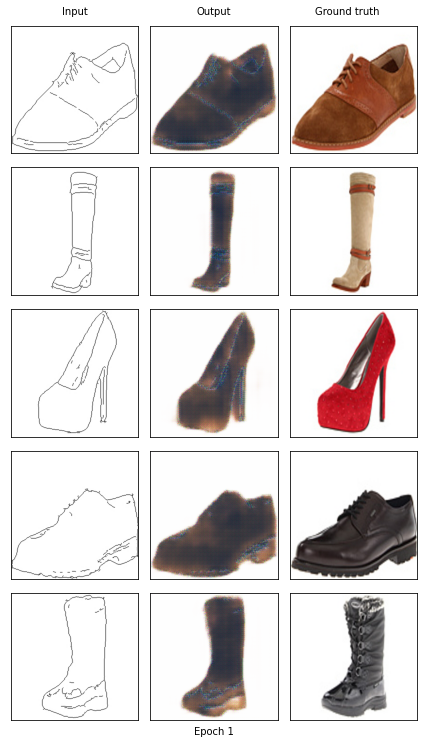
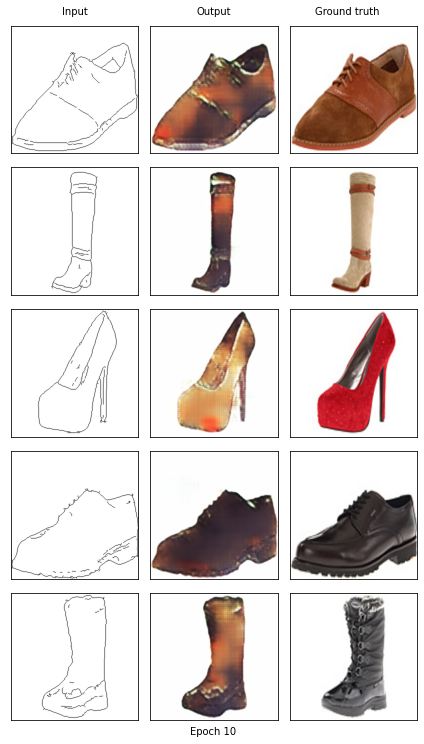
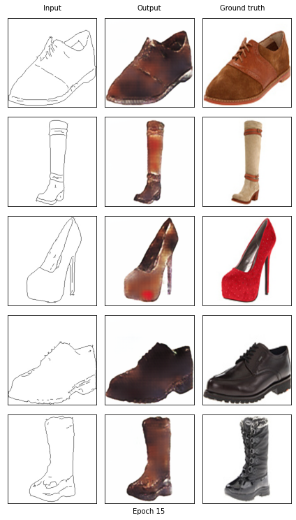
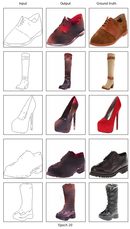
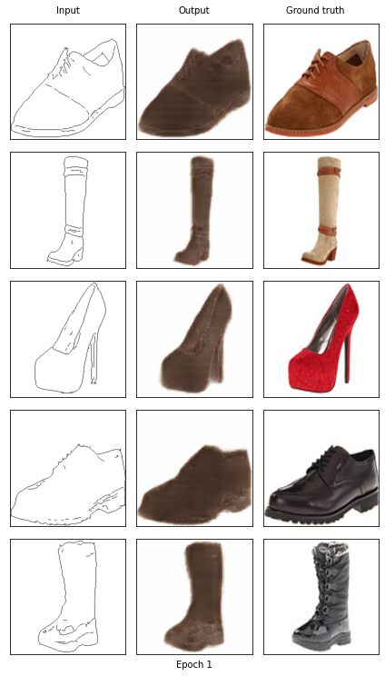
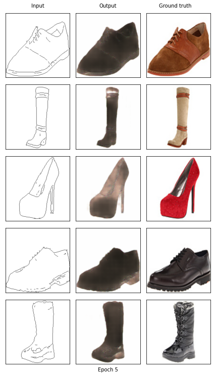
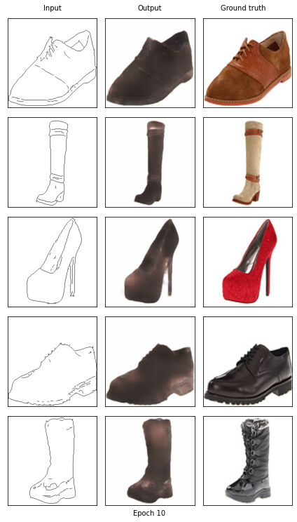
def show_result(G, x_, y_, num_epoch):
predict_images = G(x_)
fig, ax = plt.subplots(x_.size()[0], 3, figsize=(6,10))
for i in range(x_.size()[0]):
ax[i, 0].get_xaxis().set_visible(False)
ax[i, 0].get_yaxis().set_visible(False)
ax[i, 1].get_xaxis().set_visible(False)
ax[i, 1].get_yaxis().set_visible(False)
ax[i, 2].get_xaxis().set_visible(False)
ax[i, 2].get_yaxis().set_visible(False)
ax[i, 0].cla()
ax[i, 0].imshow(process_image(x_[i]))
ax[i, 1].cla()
ax[i, 1].imshow(process_image(predict_images[i]))
ax[i, 2].cla()
ax[i, 2].imshow(process_image(y_[i]))
plt.tight_layout()
label_epoch = 'Epoch {0}'.format(num_epoch)
fig.text(0.5, 0, label_epoch, ha='center')
label_input = 'Input'
fig.text(0.18, 1, label_input, ha='center')
label_output = 'Output'
fig.text(0.5, 1, label_output, ha='center')
label_truth = 'Ground truth'
fig.text(0.81, 1, label_truth, ha='center')
plt.show()
# Helper function for counting number of trainable parameters.
def count_params(model):
'''
Counts the number of trainable parameters in PyTorch.
Args:
model: PyTorch model.
Returns:
num_params: int, number of trainable parameters.
'''
num_params = sum([item.numel() for item in model.parameters() if item.requires_grad])
return num_params
# Hint: you could use following loss to complete following function
BCE_loss = nn.BCELoss().cuda()
L1_loss = nn.L1Loss().cuda()
def train(G, D, num_epochs = 20, only_L1 = False):
hist_D_losses = []
hist_G_losses = []
hist_G_L1_losses = []
###########################################################################
# TODO: Add Adam optimizer to generator and discriminator #
# You will use lr=0.0002, beta=0.5, beta2=0.999 #
###########################################################################
G_optimizer = optim.Adam(G.parameters(), betas = [0.9, 0.999], lr = 0.0002)
D_optimizer = optim.Adam(D.parameters(), betas = [0.9, 0.999], lr = 0.0002)
###########################################################################
# END OF YOUR CODE #
###########################################################################
print('training start!')
start_time = time.time()
for epoch in range(num_epochs):
print('Start training epoch %d' % (epoch + 1))
D_losses = []
G_losses = []
epoch_start_time = time.time()
num_iter = 0
for x_ in train_loader:
y_ = x_[:, :, :, img_size:]
x_ = x_[:, :, :, 0:img_size]
x_, y_ = x_.cuda(), y_.cuda()
###########################################################################
# TODO: Implement training code for the discriminator. #
# Recall that the loss is the mean of the loss for real images and fake #
# images, and made by some calculations with zeros and ones #
# We have defined the BCE_loss, which you might would like to use #
###########################################################################
D.zero_grad()
# loss for fake images
G_result = G(x_)
D_input = torch.cat([x_, G_result], 1)
D_result = D(D_input).squeeze()
D_train_loss_fake = BCE_loss(D_result, torch.zeros(D_result.size()).cuda())
# loss for real images
D_input = torch.cat([x_, y_], 1)
D_result = D(D_input).squeeze()
D_train_loss_real = BCE_loss(D_result, torch.ones(D_result.size()).cuda())
D_train_loss = (D_train_loss_fake + D_train_loss_real) / 2
D_train_loss.backward()
D_optimizer.step()
loss_D = D_train_loss.detach().item()
###########################################################################
# END OF YOUR CODE #
###########################################################################
# Train the generator
G.zero_grad()
G_result = G(x_)
D_input = torch.cat([x_, G_result], 1)
D_result = D(D_input).squeeze()
if only_L1:
G_train_loss = L1_loss(G_result, y_)
hist_G_losses.append(L1_loss(G_result, y_).detach().item())
else:
G_train_loss = BCE_loss(D_result, torch.ones(D_result.size()).cuda()) + 100 * L1_loss(G_result, y_)
hist_G_L1_losses.append(L1_loss(G_result, y_).detach().item())
hist_G_losses.append(BCE_loss(D_result, torch.ones(D_result.size()).cuda()).detach().item())
G_train_loss.backward()
G_optimizer.step()
loss_G = G_train_loss.detach().item()
D_losses.append(loss_D)
hist_D_losses.append(loss_D)
G_losses.append(loss_G)
num_iter += 1
epoch_end_time = time.time()
per_epoch_ptime = epoch_end_time - epoch_start_time
print('[%d/%d] - using time: %.2f seconds' % ((epoch + 1), num_epochs, per_epoch_ptime))
print('loss of discriminator D: %.3f' % (torch.mean(torch.FloatTensor(D_losses))))
print('loss of generator G: %.3f' % (torch.mean(torch.FloatTensor(G_losses))))
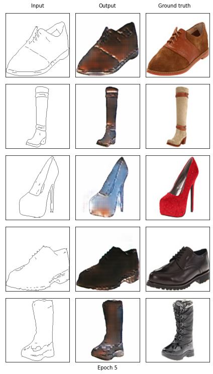
if epoch == 0 or (epoch + 1) % 5 == 0:
with torch.no_grad():
show_result(G, fixed_x_, fixed_y_, (epoch+1))
end_time = time.time()
total_ptime = end_time - start_time
return hist_D_losses, hist_G_losses, hist_G_L1_losses
In this part, train your model with c=100 with at least 20 epochs.
# Define network
G_100 = generator()
D_100 = discriminator()
G_100.weight_init(mean=0.0, std=0.02)
D_100.weight_init(mean=0.0, std=0.02)
G_100.cuda()
D_100.cuda()
G_100.train()
D_100.train()
discriminator(
  (conv1): Sequential(
    (0): Conv2d(6, 64, kernel_size=(4, 4), stride=(2, 2), padding=(1, 1))
  )
  (conv2): Sequential(
    (0): Conv2d(64, 128, kernel_size=(4, 4), stride=(2, 2), padding=(1, 1))
    (1): BatchNorm2d(128, eps=1e-05, momentum=0.1, affine=True, track_running_stats=True)
  )
  (conv3): Sequential(
    (0): Conv2d(128, 256, kernel_size=(4, 4), stride=(2, 2), padding=(1, 1))
    (1): BatchNorm2d(256, eps=1e-05, momentum=0.1, affine=True, track_running_stats=True)
  )
  (conv4): Sequential(
    (0): Conv2d(256, 512, kernel_size=(4, 4), stride=(1, 1), padding=(1, 1))
    (1): BatchNorm2d(512, eps=1e-05, momentum=0.1, affine=True, track_running_stats=True)
  )
  (conv5): Sequential(
    (0): Conv2d(512, 1, kernel_size=(4, 4), stride=(1, 1), padding=(1, 1))
  )
)
#training, you will be expecting 1-2 minutes per epoch.
# TODO: change_num_epochs if you want
hist_D_100_losses, hist_G_100_BCE_losses, hist_G_100_L1_losses = train(G_100, D_100, num_epochs = 20, only_L1 = False)
training start!
Start training epoch 1
[1/20] - using time: 74.01 seconds
loss of discriminator D: 0.415
loss of generator G: 28.001
Start training epoch 2
[2/20] - using time: 72.84 seconds
loss of discriminator D: 0.450
loss of generator G: 21.059
Start training epoch 3
[3/20] - using time: 72.62 seconds
loss of discriminator D: 0.534
loss of generator G: 19.574
Start training epoch 4
[4/20] - using time: 72.92 seconds
loss of discriminator D: 0.533
loss of generator G: 18.778
Start training epoch 5
[5/20] - using time: 72.83 seconds
loss of discriminator D: 0.510
loss of generator G: 18.047
Start training epoch 6
[6/20] - using time: 72.74 seconds
loss of discriminator D: 0.505
loss of generator G: 17.362
Start training epoch 7
[7/20] - using time: 72.69 seconds
loss of discriminator D: 0.512
loss of generator G: 16.121
Start training epoch 8
[8/20] - using time: 72.61 seconds
loss of discriminator D: 0.466
loss of generator G: 15.682
Start training epoch 9
[9/20] - using time: 72.78 seconds
loss of discriminator D: 0.480
loss of generator G: 14.794
Start training epoch 10
[10/20] - using time: 72.94 seconds
loss of discriminator D: 0.425
loss of generator G: 14.835
Start training epoch 11
[11/20] - using time: 72.34 seconds
loss of discriminator D: 0.438
loss of generator G: 14.498
Start training epoch 12
[12/20] - using time: 72.30 seconds
loss of discriminator D: 0.437
loss of generator G: 14.018
Start training epoch 13
[13/20] - using time: 72.36 seconds
loss of discriminator D: 0.449
loss of generator G: 13.288
Start training epoch 14
[14/20] - using time: 72.25 seconds
loss of discriminator D: 0.494
loss of generator G: 12.553
Start training epoch 15
[15/20] - using time: 72.21 seconds
loss of discriminator D: 0.539
loss of generator G: 11.924
Start training epoch 16
[16/20] - using time: 72.52 seconds
loss of discriminator D: 0.514
loss of generator G: 11.778
Start training epoch 17
[17/20] - using time: 72.60 seconds
loss of discriminator D: 0.573
loss of generator G: 11.079
Start training epoch 18
[18/20] - using time: 72.52 seconds
loss of discriminator D: 0.555
loss of generator G: 10.543
Start training epoch 19
[19/20] - using time: 72.57 seconds
loss of discriminator D: 0.554
loss of generator G: 10.212
Start training epoch 20
[20/20] - using time: 72.48 seconds
loss of discriminator D: 0.571
loss of generator G: 9.904
!mkdir models
torch.save(G_100.state_dict(), './models/G_100.pth')
torch.save(D_100.state_dict(), './models/D_100.pth')
In this part, train your model with only L1 loss with 10 epochs.
# Define network
G_L1 = generator()
D_L1 = discriminator()
G_L1.weight_init(mean=0.0, std=0.02)
D_L1.weight_init(mean=0.0, std=0.02)
G_L1.cuda()
D_L1.cuda()
G_L1.train()
D_L1.train()

# training
hist_D_L1_losses, hist_G_L1_losses, _ = train(G_L1, D_L1, num_epochs = 10, only_L1 = True)
training start!
Start training epoch 1
[1/10] - using time: 66.31 seconds
loss of discriminator D: 0.226
loss of generator G: 0.261
Start training epoch 2
[2/10] - using time: 66.78 seconds
loss of discriminator D: 0.096
loss of generator G: 0.186
Start training epoch 3
[3/10] - using time: 67.00 seconds
loss of discriminator D: 0.087
loss of generator G: 0.174
Start training epoch 4
[4/10] - using time: 66.82 seconds
loss of discriminator D: 0.089
loss of generator G: 0.168
Start training epoch 5
[5/10] - using time: 66.82 seconds
loss of discriminator D: 0.098
loss of generator G: 0.154
Start training epoch 6
[6/10] - using time: 66.61 seconds
loss of discriminator D: 0.022
loss of generator G: 0.149
Start training epoch 7
[7/10] - using time: 66.41 seconds
loss of discriminator D: 0.030
loss of generator G: 0.140
Start training epoch 8
[8/10] - using time: 66.53 seconds
loss of discriminator D: 0.048
loss of generator G: 0.130
Start training epoch 9
[9/10] - using time: 66.60 seconds
loss of discriminator D: 0.008
loss of generator G: 0.125
Start training epoch 10
[10/10] - using time: 66.55 seconds
loss of discriminator D: 0.001
loss of generator G: 0.119
torch.save(G_L1.state_dict(), './models/G_L1.pth')
torch.save(D_L1.state_dict(), './models/D_L1.pth')
The following cell saves the trained model parameters to your Google Drive so you could reuse those parameters later without retraining.
from google.colab import drive
drive.mount('/content/drive')
!cp "./models/" -r "/content/drive/My Drive/"
Mounted at /content/drive
TODO: Please comment on the quality of generated images from L1+cGAN and L1 only:
When we use L1 + cGan, the generated images become more and more colorful with training. Aftoer 20 epoch, generated images are quite colorful like real shoes. However, when we only use L1, the generated images are just all brown even though we keep training the model.
Step 4: Visualization
Please plot the generator BCE and L1 losses, as well as the discriminator loss. For this, please use c=100, and use 3 separate plots.
len(hist_G_100_BCE_losses)
5000
###########################################################################
# TODO: Plot the G/D loss history (y axis) vs. Iteration (x axis)         #
# You will have three plots, with hist_D_100_losses,                      #
# hist_G_100_BCE_losses, hist_G_100_L1_losses respectively.               #
# Hiint: Use plt.legend if you want visualize the annotation for your     #
# curve                                                                   #
###########################################################################
x = np.arange(len(hist_G_100_BCE_losses))
# hist_D_100_losses, hist_G_100_BCE_losses, hist_G_100_L1_losses = train(G_100, D_100, num_epochs = 20, only_L1 = False)
# hist_D_L1_losses, hist_G_L1_losses, _ = train(G_L1, D_L1, num_epochs = 10, only_L1 = True)

# generator BCE losses
plt.figure()
plt.plot(x, hist_G_100_BCE_losses)
plt.xlabel('Iteration')
plt.ylabel('Generator BCE losses')
plt.title('G100 BCE loss history')
plt.show()

# generator L1 losses
plt.plot(x, hist_G_100_L1_losses)
plt.xlabel('Iteration')
plt.ylabel('Generator L1 losses')
plt.title('G100 L1 loss history')
plt.show()

# discriminator loss
plt.plot(x, hist_D_100_losses)
plt.xlabel('Iteration')
plt.ylabel('Discriminator losses')
plt.title('D100 loss history')
plt.show()

###########################################################################
#                              END OF YOUR CODE                           #
###########################################################################


In this section, plot the G/D loss history vs. Iteration of model with only L1 loss in 2 seperate plots.
###########################################################################
# TODO: Plot the G/D loss history vs. Iteration in one plot               #
# You will have two plots, with hist_G_L1_losses and hist_D_L1_losses     #
# respectively                                                            #
###########################################################################

x = np.arange(len(hist_G_L1_losses))


# generator L1 losses
plt.plot(x, hist_G_L1_losses)
plt.xlabel('Iteration')
plt.ylabel('Generator losses')
plt.title('G_L1 loss history')
plt.show()

# discriminator loss
plt.plot(x, hist_D_L1_losses)
plt.xlabel('Iteration')
plt.ylabel('Discriminator losses')
plt.title('D_L1 loss history')
plt.show()

###########################################################################
#                              END OF YOUR CODE                           #
###########################################################################
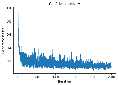
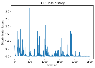
TODO: Please comment on the loss plots for L1+cGAN and L1 only models:
The BCE loss of generator fluctuates only within a certain range, while the L1 loss of generator tends to decrease steadily. Also, loss of generator for L1 + cGan model fluctuates only within a certain range, but loss of generator for L1 only model do not show such a regular trend.
Step 5: Design Your Shoe
After the pix2pix model has been trained on this dataset, we can apply the trained generative model to translate any user-provided sketch to a synthetic image. Please draw a shoe in the sketch panel we provide in the Colab notebook and translate it to a shoe image with the trained model. Feel free to post your generated image to a Piazza thread.
# Build a panel that allows sketching in Colab
# Source: https://gist.github.com/korakot/8409b3feec20f159d8a50b0a811d3bca
from IPython.display import HTML, Image
from google.colab.output import eval_js
from base64 import b64decode
from PIL import Image

canvas_html = """
<canvas width=%d height=%d></canvas>
<button>Finish</button>
<script>
var canvas = document.querySelector('canvas')
var ctx = canvas.getContext('2d')
ctx.lineWidth = %d
var button = document.querySelector('button')
var mouse = {x: 0, y: 0}

canvas.addEventListener('mousemove', function(e) {
  mouse.x = e.pageX - this.offsetLeft
  mouse.y = e.pageY - this.offsetTop
})
canvas.onmousedown = ()=>{
  ctx.beginPath()
  ctx.moveTo(mouse.x, mouse.y)
  canvas.addEventListener('mousemove', onPaint)
}
canvas.onmouseup = ()=>{
  canvas.removeEventListener('mousemove', onPaint)
}
var onPaint = ()=>{
  ctx.lineTo(mouse.x, mouse.y)
  ctx.stroke()
}

var data = new Promise(resolve=>{
  button.onclick = ()=>{
    resolve(canvas.toDataURL('image/png'))
  }
})
</script>
"""

def draw(filename='drawing.png', w=400, h=200, line_width=1):
  print('Please sketch below.')
  display(HTML(canvas_html % (w, h, line_width)))
  data = eval_js("data")
  binary = b64decode(data.split(',')[1])
  with open(filename, 'wb') as f:
      f.write(binary)
  return len(binary)

!mkdir mini-edges2shoes/custom
!apt-get --quiet install imagemagick
# Press left mouse button and drag your mouse to draw a sketch.
# Then click Finish.
draw(w=256, h=256)
!convert drawing.png drawing.jpg

# save the drawing to dataset folder as a jpg image
img = np.asarray(Image.open('drawing.png'))
img = 255 - img

image.imsave('./mini-edges2shoes/custom/drawing.jpg', np.repeat(img[:,:,3:], 3, axis=2))
custom_dt = Edges2Image('./mini-edges2shoes', 'custom', transform)
custom_loader = DataLoader(custom_dt, batch_size=1, shuffle=False)
Run the following cell to mount your Google Drive. You can retrieve your saved model parameters from your Google Drive.
from google.colab import drive
drive.mount('/content/drive')
# Optional: for loading saved generator
G_100 = generator().cuda()
# For retrieving the model saved to Google Drive
# TODO: add your notebook path
path = None
if path:
  G_100.load_state_dict(torch.load(path + 'models/G_100.pth'))
else:
  G_100.load_state_dict(torch.load('/content/drive/My Drive/models/G_100.pth'))
# For retreiving the model saved on Colab (you just finished training)

G_100.eval()

# process the sketch
for x_ in custom_loader:
  x_ = x_.cuda()[:,:,:,:img_size]
  y_ = G_100(x_)

# visualize the image
fig, axis = plt.subplots(1, 2, figsize=(10, 5))
img_ = process_image(y_[0])
img = process_image(x_[0])
axis[0].imshow(img)
axis[0].axis('off')
axis[1].imshow(img_)
axis[1].axis('off')
plt.show()
Problem 2: Understanding pix2pix - calculating receptive field size
The network architecture that we used in the previous section is often called a PatchGAN. This is because the discriminator classifies individual image patches, rather than assigning a score to a whole image. To help you better understand the concept of classifying on a patch level, we calculate the patch size. This is equivalent to the receptive field size of the final convolutional layer of the network
Please write down the receptive field size in in this text cell. The receptive field size is calculated with:
\[r_i = r_{i-1} + ((k_i - 1) * \prod_{j=0}^{i-1}s_j)\]where $k$ is the kernel size of current layer, $s_j$ is the stride of $j^{th}$ layer, and $r_i$ is the receptive field size of $i^{th}$ layer.
We have $r_0 = 1, s_0 = 1$. The kernel size for all layers in the discriminator is 4, and the stride is 2.
The receptive of C64, C128, C256, C512 is $r_1, r_2, r_3, r_4$ respectively.
Please directly replace $?$ with you answer in the expression below.
\(Input\) \(\downarrow\) \(C64 (r_1) (\text{receptive field size} = 4)\) \(\downarrow\) \(C128(r_2)(\text{receptive field size}= 10)\) \(\downarrow\) \(C256(r_3)(\text{receptive field size}= 22)\) \(\downarrow\) \(C512(r_4)(\text{receptive field size}= 46)\)
Problem 3: Style transfer (EECS 504)
Step 0: Downloading the dataset and backbone network.
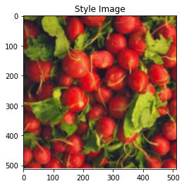
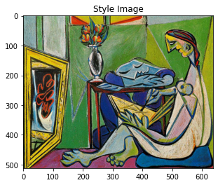
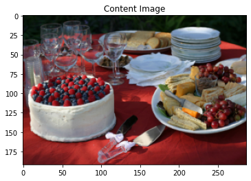
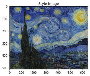
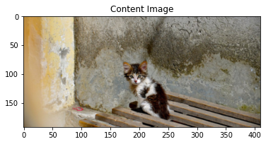
In this problem, we will implement the loss functions for the neural artistic style transfer method of Gatys et al. We take two images as input: one that defines the content and another that defines the style. We have provided five paintings that define the styles, and images COCO that define the content.
![]()
Two losses are needed to accomplish style transfer: the content loss and the style loss. Both losses are calculated between the input image (the same as content image or a random noise) and the reference image (style/content).
For this problem, we will use five images as our artistic style, and the Coco validation set as our content image.
A pretrained SqueezeNet will be applied to extract features.
if os.path.isdir('styles') and os.path.isdir('contents'):
  print('Style images exist')
else:
  print('Downloading images')
  # Download style images
  !wget https://eecs.umich.edu/courses/eecs442-ahowens/fa22/data/style_images.zip
  !unzip style_images.zip && rm style_images.zip

  # Download content images
  !wget http://images.cocodataset.org/zips/val2017.zip
  !unzip -q val2017.zip && rm val2017.zip
  !mkdir contents
  !mv val2017/* ./contents/

# Download the model
cnn = torchvision.models.squeezenet1_1(pretrained=True).features
cnn = cnn.to(device)

# Freeze the parameters as there's no need to train the net. Ignore the warnings.
for param in cnn.parameters():
    param.requires_grad = False
Style images exist


/usr/local/lib/python3.7/dist-packages/torchvision/models/_utils.py:209: UserWarning: The parameter 'pretrained' is deprecated since 0.13 and will be removed in 0.15, please use 'weights' instead.
  f"The parameter '{pretrained_param}' is deprecated since 0.13 and will be removed in 0.15, "
/usr/local/lib/python3.7/dist-packages/torchvision/models/_utils.py:223: UserWarning: Arguments other than a weight enum or `None` for 'weights' are deprecated since 0.13 and will be removed in 0.15. The current behavior is equivalent to passing `weights=SqueezeNet1_1_Weights.IMAGENET1K_V1`. You can also use `weights=SqueezeNet1_1_Weights.DEFAULT` to get the most up-to-date weights.
  warnings.warn(msg)
Step 1: Create the image loader and some utility funtions
We provide the dataloader for images and a function to get the list of feature maps from a forward pass in the network.
# Dataloader
imsize = 512
SQUEEZENET_MEAN = torch.tensor([0.485, 0.456, 0.406], dtype=torch.float)
SQUEEZENET_STD = torch.tensor([0.229, 0.224, 0.225], dtype=torch.float)
def image_loader(image_name, imsize):
image = Image.open(image_name)
transform = transforms.Compose([
transforms.Resize(imsize),
transforms.ToTensor(),
transforms.Normalize(mean=SQUEEZENET_MEAN.tolist(), std=SQUEEZENET_STD.tolist()),
transforms.Lambda(lambda x: x[None]),
])
image = transform(image)
return image.to(device, torch.float)
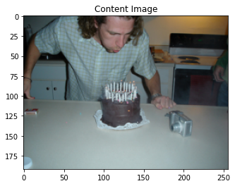
# visualizing the content and style images
style_img = image_loader("styles/muse.jpg", imsize)
content_img = image_loader("contents/000000211825.jpg", imsize)
def deprocess(img):
transform = transforms.Compose(
[
transforms.Lambda(lambda x: x[0]),
transforms.Normalize(mean=[0, 0, 0], std=(1.0 / SQUEEZENET_STD).tolist()),
transforms.Normalize(mean=(-SQUEEZENET_MEAN).tolist(), std=[1, 1, 1]),
transforms.Lambda(lambda x: x),
transforms.ToPILImage(),
]
)
return transform(img)
plt.ion()
def imshow(im_tensor, title=None):
image = im_tensor.cpu().clone()
image = deprocess(image)
plt.imshow(image)
if title is not None:
plt.title(title)
plt.pause(0.001)
plt.figure()
imshow(style_img, title='Style Image')
plt.figure()
imshow(content_img, title='Content Image')


def get_feature_maps(x, cnn):
    """
    Get the list of feature maps in a forward pass.

    Inputs:
    - x: A batch of images with shape (B, C, H, W)
    - cnn: A PyTorch model that we will use to extract features.

    Returns:
    - features: A list of features for the input images x extracted using the cnn model.
      features[i] is a Tensor of shape (B, C_i, H_i, W_i).
    """
    feats = []
    in_feat = x
    for layer in cnn._modules.values():
        out_feat = layer(in_feat)
        feats.append(out_feat)
        in_feat = out_feat
    return feats
Step 2: Implementing content loss
First, we will implement the {\em content loss}. This loss encourages the generated image to match the scene structure of the content image. We will implement this loss as the squared $\ell_2$ distance between two convolutional feature maps. Given a feature map of input image $F^x$ and the feature map of content image $F^{c}$, both of shape $(C, H, W)$, the content loss is calculated as follows:
\begin{equation} \mathcal{L}c = \sum{c,i,j}(F^{c}{c, i, j} - F^{x}{c, i, j}) ^ 2. \end{equation}
def content_loss(f_x, f_con):
    """
    Compute the gram matrix without loop.

    Inputs:
    - f_x: features of the input image with size (1, C, H, W).
    - f_cont: features of the content image with size (1, C, H, W).
    Returns:
    - lc: the content loss
    """

    lc = None

    ###########################################################################
    # TODO: Implement the content loss.                                       #
    # You can check your content loss with some code blocks below             #
    ###########################################################################

    lc = torch.sum((f_con - f_x)**2)

    ###########################################################################
    #                              END OF YOUR CODE                           #
    ###########################################################################

    return lc
Step 3: Implementing style loss
Next, we will implement the {\em style loss}. This loss encourages the texture of the resulting image to match the input style image. We compute a weighted, squared $\ell_2$ distance between Gram matrices for several layers of the network.
The first step is to calculate the Gram matrix. Given a feature map $F$ of size $(C, H, W)$, the Gram matrix $G \in \mathbb{R}^{C \times C}$ computes the sum of products between channels. The entries $k, l$ of the matrix are computed as: \begin{equation} G_{k,l} = \sum_{i,j} F_{k,i,j} F_{l,i,j}. \end{equation}
The second step is to compare the generated image’s Gram matrix with that of the input style image. Define the Gram matrix of input image feature map and style image feature map of at the $l^{th}$ layer as $G^{x,l}$ and $G^{s, l}$, and the weight of the layer as $w^l$. Style loss at the $l^{th}$ layer is \begin{equation} L_s^l = w^l \sum_{i,j} (G^{x,l}{i,j} - G^{s, l}{i,j})^2, \end{equation} where $w^l$ is the weight of layer $l$. The total style loss is a sum over all style layers: \begin{equation} \mathcal{L}_s = \sum_l L_s^l. \end{equation}
def gram_matrix(feat, normalize = True):
    """
    Compute the gram matrix.

    Inputs:
    - feat: a feature tensor of shape (1, C, H, W).
    - normalize: if normalize is true, divide the gram matrix by C*H*W:
    Returns
    - gram: the tram matrix
    """

    gram = None

    ###########################################################################
    # TODO: Implement the gram matrix. You should not use a loop or           #
    # comprehension                                                           #
    ###########################################################################
    B, C, H, W = feat.shape
    gram = torch.zeros([C, C])

    # for i in np.arange(C):
    #   for j in np.arange(C):
    #     gram[i, j] = torch.sum(torch.mul(feat[:,i,:,:], feat[:,j,:,:]))
    feat = feat.view(B, C, H * W)
    gram = feat.bmm(feat.transpose(1, 2))

    if normalize:
      gram = gram / (C * H * W)


    ###########################################################################
    #                              END OF YOUR CODE                           #
    ###########################################################################

    return gram
# Test your gram matrix, you should be expecting a difference smaller than 0.001
t1 = torch.arange(8).reshape(1,2,2,2)
result = torch.tensor([[[ 1.7500,  4.7500],[ 4.7500, 15.7500]]])
print(((gram_matrix(t1) - result)**2).sum().item())
0.0
def style_loss(feats, style_layers, style_targets, style_weights):
    """
    Computes the style loss at a set of layers.

    Inputs:
    - feats: list of the features at every layer of the current image, as produced by
      the extract_features function. The list will contain the features of all layers
      instead of the layers for calcculating style loss
    - style_layers: List of layer indices into feats giving the layers to include in the
      style loss.
    - style_targets: List of the same length as style_layers, where style_targets[i] is
      a PyTorch Tensor giving the Gram matrix of the source style image computed at
      layer style_layers[i].
    - style_weights: List of the same length as style_layers, where style_weights[i]
      is a scalar giving the weight for the style loss at layer style_layers[i].

    Returns:
    - loss: A PyTorch Tensor holding a scalar giving the style loss.
    """

    loss = None

    ###########################################################################
    # TODO: Implement the style loss                                          #
    # You can check your style loss with some code blocks below               #
    ###########################################################################
    loss = 0.0

    for l in np.arange(len(style_layers)):
      gram_img_l = gram_matrix(feats[style_layers[l]])
      loss += style_weights[l] * torch.sum((gram_img_l - style_targets[l]) ** 2)

    ###########################################################################
    #                              END OF YOUR CODE                           #
    ###########################################################################

    return loss
Step 4: Network Training
Finally, we will try varying the layer used to compute the content loss. Try several different layers l = 0, 1, 2, …, 12 and report which one gave you the best qualitative results.
def style_transfer(content_image, style_image, image_size, style_size, content_layer, content_weight,
style_layers, style_weights, init_random = False):
"""
Run style transfer!
Inputs:
- content_image: filename of content image
- style_image: filename of style image
- image_size: size of smallest image dimension (used for content loss and generated image)
- style_size: size of smallest style image dimension
- content_layer: layer to use for content loss
- content_weight: weighting on content loss
- style_layers: list of layers to use for style loss
- style_weights: list of weights to use for each layer in style_layers
- init_random: initialize the starting image to uniform random noise
"""
# Extract features for the content image
content_img = image_loader(content_image, image_size)
feats = get_feature_maps(content_img, cnn)
content_target = feats[content_layer].clone()
# Extract features for the style image
style_img = image_loader(style_image, style_size)
feats = get_feature_maps(style_img, cnn)
style_targets = []
for idx in style_layers:
style_targets.append(gram_matrix(feats[idx].clone()))
# Initialize output image to content image or nois
if init_random:
img = torch.Tensor(content_img.size()).uniform_(0, 1).to(device)
else:
img = content_img.clone().to(device)
# We do want the gradient computed on our image!
img.requires_grad_()
# Set up optimization hyperparameters
initial_lr = 1
decayed_lr = 0.1
decay_lr_at = 180
# Note that we are optimizing the pixel values of the image by passing
# in the img Torch tensor, whose requires_grad flag is set to True
optimizer = torch.optim.Adam([img], lr=initial_lr)
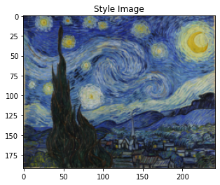
plt.figure()
imshow(style_img, title='Style Image')
plt.figure()
imshow(content_img, title='Content Image')
for t in range(200):
if t < 190:
img.data.clamp_(-1.5, 1.5)
optimizer.zero_grad()
feats = get_feature_maps(img, cnn)
# Compute loss
c_loss = content_loss(feats[content_layer], content_target) * content_weight
s_loss = style_loss(feats, style_layers, style_targets, style_weights)
loss = c_loss + s_loss
loss.backward()
# Perform gradient descents on our image values
if t == decay_lr_at:
optimizer = torch.optim.Adam([img], lr=decayed_lr)
optimizer.step()
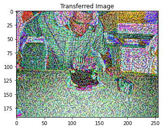
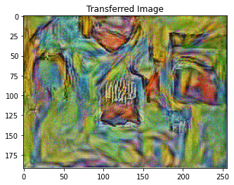
if t % 100 == 0:
print('Iteration {}'.format(t))
plt.figure()
imshow(img, title='Transferred Image')
plt.show()
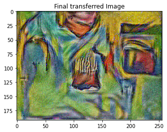
print('Iteration {}'.format(t))
plt.figure()
imshow(img, title='Final transferred Image')
# Check of content loss. Ignore the style image.
params_content_check = {
    'content_image':'contents/000000211825.jpg',
    'style_image':'styles/muse.jpg',
    'image_size':192,
    'style_size':512,
    'content_layer':2,
    'content_weight':3e-2,
    'style_layers':[1, 4, 6, 7],
    'style_weights':[0, 0, 0, 0],
    'init_random': True
}

style_transfer(**params_content_check)


Iteration 0

Iteration 100

Iteration 199

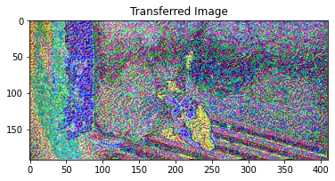
# Check of style loss. You should see the texture of the image. Ignore the content image.
params_style_check = {
    'content_image':'contents/000000211825.jpg',
    'style_image':'styles/texture.jpg',
    'image_size':192,
    'style_size':512,
    'content_layer':2,
    'content_weight':0,
    'style_layers':[0, 1],
    'style_weights':[200000, 200000],
    'init_random': True
}

style_transfer(**params_style_check)

Iteration 0

Iteration 100

Iteration 199

params1 = {
    'content_image':'contents/000000211825.jpg',
    'style_image':'styles/muse.jpg',
    'image_size':192,
    'style_size':512,
    'content_layer':2,
    'content_weight':3e-2,
    'style_layers':[1, 4, 6, 7],
    'style_weights':[200000, 800, 12, 1],
}

style_transfer(**params1)
Iteration 0
Iteration 100
Iteration 199
params2 = {
    'content_image':'contents/000000118515.jpg',
    'style_image':'styles/starry_night.jpg',
    'image_size':192,
    'style_size':192,
    'content_layer':3,
    'content_weight':3e-2,
    'style_layers':[1, 4, 6, 7],
    'style_weights':[200000, 800, 12, 1],
}

style_transfer(**params2)

Iteration 0

Iteration 100

Iteration 199

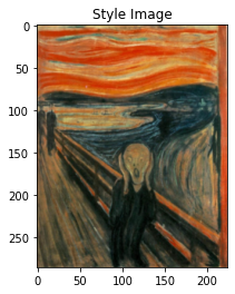
params3 = {
    'content_image':'contents/000000002157.jpg',
    'style_image':'styles/the_scream.jpg',
    'image_size':192,
    'style_size':224,
    'content_layer':2,
    'content_weight':3e-2,
    'style_layers':[1, 4, 6, 7],
    'style_weights':[200000, 800, 12, 1],
}

style_transfer(**params3)

# Feel free ot change the images and get your own style transferred image
Iteration 0

Iteration 100

Iteration 199

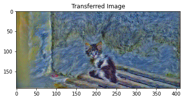
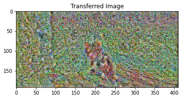
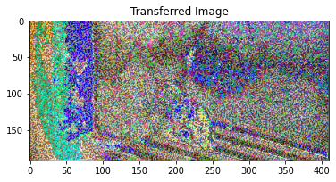
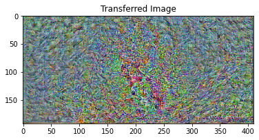
TODO: Finally, we will try varying the layer used to compute the content loss. Try different layers l = 0, 1, 2, …, 12 and report which one provides the best qualitative results.
The closer the content layer is to 12, the harder it is to check the content img. When I used the first layer, I was able to override the style while best preserving the content image.
params_1 = {
    'content_image':'contents/000000118515.jpg',
    'style_image':'styles/starry_night.jpg',
    'image_size':192,
    'style_size':512,
    'content_layer':1,
    'content_weight':3e-2,
    'style_layers':[1, 4, 6, 7],
    'style_weights':[200000, 800, 12, 1],
}

style_transfer(**params_1)


Iteration 0

Iteration 100

Iteration 199

params_3 = {
    'content_image':'contents/000000118515.jpg',
    'style_image':'styles/starry_night.jpg',
    'image_size':192,
    'style_size':512,
    'content_layer':3,
    'content_weight':3e-2,
    'style_layers':[1, 4, 6, 7],
    'style_weights':[200000, 800, 12, 1],
}

style_transfer(**params_3)


Iteration 0
Iteration 100
Iteration 199

params_4 = {
    'content_image':'contents/000000118515.jpg',
    'style_image':'styles/starry_night.jpg',
    'image_size':192,
    'style_size':512,
    'content_layer':4,
    'content_weight':3e-2,
    'style_layers':[1, 4, 6, 7],
    'style_weights':[200000, 800, 12, 1],
}

style_transfer(**params_4)


Iteration 0

Iteration 100

Iteration 199

params_5 = {
    'content_image':'contents/000000118515.jpg',
    'style_image':'styles/starry_night.jpg',
    'image_size':192,
    'style_size':512,
    'content_layer':5,
    'content_weight':3e-2,
    'style_layers':[1, 4, 6, 7],
    'style_weights':[200000, 800, 12, 1],
}

style_transfer(**params_5)

Iteration 0

Iteration 100

Iteration 199

params_6 = {
    'content_image':'contents/000000118515.jpg',
    'style_image':'styles/starry_night.jpg',
    'image_size':192,
    'style_size':512,
    'content_layer':6,
    'content_weight':3e-2,
    'style_layers':[1, 4, 6, 7],
    'style_weights':[200000, 800, 12, 1],
}

style_transfer(**params_6)


Iteration 0

Iteration 100

Iteration 199

params_9 = {
    'content_image':'contents/000000118515.jpg',
    'style_image':'styles/starry_night.jpg',
    'image_size':192,
    'style_size':512,
    'content_layer':9,
    'content_weight':3e-2,
    'style_layers':[1, 4, 6, 7],
    'style_weights':[200000, 800, 12, 1],
}

style_transfer(**params_9)


Iteration 0

Iteration 100
Iteration 199

params_12 = {
    'content_image':'contents/000000118515.jpg',
    'style_image':'styles/starry_night.jpg',
    'image_size':192,
    'style_size':512,
    'content_layer':12,
    'content_weight':3e-2,
    'style_layers':[1, 4, 6, 7],
    'style_weights':[200000, 800, 12, 1],
}

style_transfer(**params_12)

Iteration 0
Iteration 100
Iteration 199
