HW7. Machine Learning 2: Classification

Topics: K-NN, Linear SVM, RBF SVM, Gaussian process classifier, Decision tree classifier, Randomforest classifer, Neural network, AdaBoost classifer, Gaussian naive bayes classifer, PCA, t-SNE

---

This is, perhaps, one of the most exciting homework assignments that you have encountered in this course!

You are going to try your hand at a Kaggle competition to predict Titanic survivorship. (Recall that we’ve played with Titanic data earlier in this course – this data set is slightly different.)

(NOTE: if you prefer to not submit your work to the Kaggle competition that’s fine – just contact Chris via email (cteplovs@umich.edu) and we will work out an alternative.)

To start with, make sure you have a Kaggle account, then navigate to the Titanic: Machine Learning from Disaster project page.

We’ll view the introductory video together in class.

The basic steps for this assignment are outlined in the video:

1. Accept the rules and join the competition
2. Download the data (from the data tab of the competition page)
3. Understand the problem
4. EDA (Exploratory Data Analysis)
5. Train, tune, and ensemble (!) your machine learning models
6. Upload your prediction as a submission on Kaggle and receive an accuracy score

additionally, you will

1. Upload your final notebook to Canvas and report your best accuracy score.

Note that class grades are not entirely dependent on your accuracy score.
All models that achieve 75% accuracy will receive full points for the accuracy component of this assignment.

Rubric:

1. (20 points) EDA
2. (60 points) Train, tune, and ensemble machine learning models
3. (10 points) Accuracy score based on Kaggle submission report (or alternative, see NOTE above).
4. (10 points) PEP-8, grammar, spelling, style, etc.

Some additional notes:

1. If you use another notebook, code, or approaches be sure to reference the original work. (Note that we recommend you study existing Kaggle notebooks before starting your own work.)
2. You can help each other but in the end you must submit your own work, both to Kaggle and to Canvas.

Some additional resources:

• “ensemble” your models with a VotingClassifier
• a good primer on feature engineering
• There are a lot of good notebooks to study (check the number of upvotes to help guide your exploration)

(and don’t cheat)

One final note: Your submission should be a self-contained notebook that is NOT based on this one. Studying the existing Kaggle competition notebooks should give you a sense of what makes a “good” notebook.

import pandas as pd
import numpy as np
import matplotlib.pyplot as plt
import seaborn as sns
import matplotlib.patches as mpatches
import plotly.graph_objects as gp
from sklearn.model_selection import train_test_split
from sklearn.pipeline import Pipeline
from sklearn.preprocessing import StandardScaler, OneHotEncoder
from sklearn.impute import SimpleImputer
from sklearn.compose import ColumnTransformer
from sklearn.model_selection import cross_validate
from sklearn.linear_model import LinearRegression
from sklearn.metrics import mean_squared_error
import statistics
from sklearn.neural_network import MLPClassifier
from sklearn.neighbors import KNeighborsClassifier
from sklearn.svm import SVC
from sklearn.gaussian_process import GaussianProcessClassifier
from sklearn.gaussian_process.kernels import RBF
from sklearn.tree import DecisionTreeClassifier
from sklearn.ensemble import RandomForestClassifier, AdaBoostClassifier, VotingClassifier
from sklearn.naive_bayes import GaussianNB
from sklearn.discriminant_analysis import QuadraticDiscriminantAnalysis
from sklearn.decomposition import PCA
from sklearn.manifold import TSNE
from sklearn.model_selection import GridSearchCV
from sklearn.gaussian_process.kernels import RBF
from sklearn.gaussian_process.kernels import DotProduct
from sklearn.gaussian_process.kernels import Matern
from sklearn.gaussian_process.kernels import RationalQuadratic
from sklearn.gaussian_process.kernels import WhiteKernel
import warnings

warnings.filterwarnings("ignore")

sns.set(style = "darkgrid")

1. EDA

titanic = pd.read_csv("./data/titanic_train.csv")

titanic.head()

	PassengerId	Survived	Pclass	Name	Sex	Age	SibSp	Parch	Ticket	Fare	Cabin	Embarked
0	1	0	3	Braund, Mr. Owen Harris	male	22.0	1	0	A/5 21171	7.2500	NaN	S
1	2	1	1	Cumings, Mrs. John Bradley (Florence Briggs Th...	female	38.0	1	0	PC 17599	71.2833	C85	C
2	3	1	3	Heikkinen, Miss. Laina	female	26.0	0	0	STON/O2. 3101282	7.9250	NaN	S
3	4	1	1	Futrelle, Mrs. Jacques Heath (Lily May Peel)	female	35.0	1	0	113803	53.1000	C123	S
4	5	0	3	Allen, Mr. William Henry	male	35.0	0	0	373450	8.0500	NaN	S

There is a total of 12 columns, but since PassengerId is just an ID, so let’s delete the column.

titanic_id = titanic["PassengerId"]
titanic.drop("PassengerId", axis = 1, inplace = True)
titanic.head()

	Survived	Pclass	Name	Sex	Age	SibSp	Parch	Ticket	Fare	Cabin	Embarked
0	0	3	Braund, Mr. Owen Harris	male	22.0	1	0	A/5 21171	7.2500	NaN	S
1	1	1	Cumings, Mrs. John Bradley (Florence Briggs Th...	female	38.0	1	0	PC 17599	71.2833	C85	C
2	1	3	Heikkinen, Miss. Laina	female	26.0	0	0	STON/O2. 3101282	7.9250	NaN	S
3	1	1	Futrelle, Mrs. Jacques Heath (Lily May Peel)	female	35.0	1	0	113803	53.1000	C123	S
4	0	3	Allen, Mr. William Henry	male	35.0	0	0	373450	8.0500	NaN	S

There are 10 independent variables and 1 dependent variable.

• Dependent variable: Survived
• Independent variables:
  • Pclass: Ticket class. (1 = 1st, 2 = 2nd, 3 = 3rd)
  • Name
  • Sex
  • Age
  • SibSp: # of siblings / spouses aboard the Titanic
  • Parch: # of parents / children aboard the Titanic
  • Ticket: Ticket numberc
  • Fare: Passenger fare
  • Cabin: Cabin number
  • Embarked: Port of Embarkation (C = Cherbourg, Q = Queenstown, S = Southampton)

And we can categorize independent variables into 3 different categories:

• Ticket related columns: Pclass, Ticket, Fare, Cabin, Embarked
• Person related columns: Name, Sex, Age
• Family related columns: SibSp, Parch

1.0. Change column names

For just convenience, let’s change the column names.

• Dependent variable: Survived -> is_survived
• Independent variables:
  • Pclass: Ticket class. (1 = 1st, 2 = 2nd, 3 = 3rd) -> p_class
  • Name -> name
  • Sex -> sex
  • Age -> age
  • SibSp: # of siblings / spouses aboard the Titanic -> num_sb_sp
  • Parch: # of parents / children aboard the Titanic -> num_pr_ch
  • Ticket: Ticket number -> ticket_number
  • Fare: Passenger fare -> ticket_fare
  • Cabin: Cabin number -> cabin_number
  • Embarked: Port of Embarkation (C = Cherbourg, Q = Queenstown, S = Southampton) -> embark_port

titanic.rename(columns = {"Survived" : "is_survived", 
                          "Pclass" : "p_class",
                          "Name" : "name",
                          "Sex" : "sex", 
                          "Age" : "age",
                          "SibSp" : "num_sb_sp",
                          "Parch" : "num_pr_ch",
                          "Ticket" : "ticket_number",
                          "Fare" : "ticket_fare",
                          "Cabin" : "cabin_number",
                          "Embarked" : "embark_port"}, inplace = True)
titanic.head()

	is_survived	p_class	name	sex	age	num_sb_sp	num_pr_ch	ticket_number	ticket_fare	cabin_number	embark_port
0	0	3	Braund, Mr. Owen Harris	male	22.0	1	0	A/5 21171	7.2500	NaN	S
1	1	1	Cumings, Mrs. John Bradley (Florence Briggs Th...	female	38.0	1	0	PC 17599	71.2833	C85	C
2	1	3	Heikkinen, Miss. Laina	female	26.0	0	0	STON/O2. 3101282	7.9250	NaN	S
3	1	1	Futrelle, Mrs. Jacques Heath (Lily May Peel)	female	35.0	1	0	113803	53.1000	C123	S
4	0	3	Allen, Mr. William Henry	male	35.0	0	0	373450	8.0500	NaN	S

1.1. Check missing values

np.sum(titanic.isnull(), axis = 0).sort_values(ascending = False)

cabin_number     687
age              177
embark_port        2
is_survived        0
p_class            0
name               0
sex                0
num_sb_sp          0
num_pr_ch          0
ticket_number      0
ticket_fare        0
dtype: int64

• Almost every row doesn’t have a cabin_number value.
• age is the next most missing column.
• embark_port only has 2 missing values.

1.1. Ticket related columns: p_class, ticket_number, ticket_fare, cabin_number, embark_port

p_class

titanic["p_class"].value_counts()

3    491
1    216
2    184
Name: p_class, dtype: int64

• 1st class passengers: 216
• 2nd class passengers: 184
• 3rd class passengers: 491

np.sum(titanic["p_class"].isnull())

0

• There is no missing value in the p_class column

p_class ~ is_survived

Let’s check the relationship between p_class and is_survived.

p_class_is_survived = titanic.groupby(["p_class","is_survived"]).count().name.unstack().reset_index()
p_class_is_survived = p_class_is_survived.rename_axis(None, axis = 1)
p_class_is_survived["total"] = p_class_is_survived[0] + p_class_is_survived[1]
p_class_is_survived["ratio"] = np.round(p_class_is_survived[1] / p_class_is_survived.total, 2)
p_class_is_survived

	p_class	0	1	total	ratio
0	1	80	136	216	0.63
1	2	97	87	184	0.47
2	3	372	119	491	0.24

plt.figure(figsize = (14, 8))

# bar graph for total students
color = "darkblue"
ax1 = sns.barplot(x = "p_class", y = "total", color = color, alpha = 0.8, \
                  data = p_class_is_survived)
top_bar = mpatches.Patch(color = color, label = 'Num of total passengers')

# bar graph for students have research experience
color = "lightblue"
ax2 = sns.barplot(x = "p_class", y = 1,  color = color, alpha = 0.8, \
                  data = p_class_is_survived)
ax2.set_xlabel("Passenger class", fontsize = 16)
ax2.set_ylabel("Number of passengers", fontsize = 16)
low_bar = mpatches.Patch(color = color, label = 'Num of survived passengers')

# ratio
plt.text(s = "63%", x = -0.05, y = 110, fontsize = 16)
plt.text(s = "47%", x = 0.95, y = 60, fontsize = 16)
plt.text(s = "24%", x = 1.95, y = 92, fontsize = 16)

plt.legend(handles=[top_bar, low_bar])
plt.show()

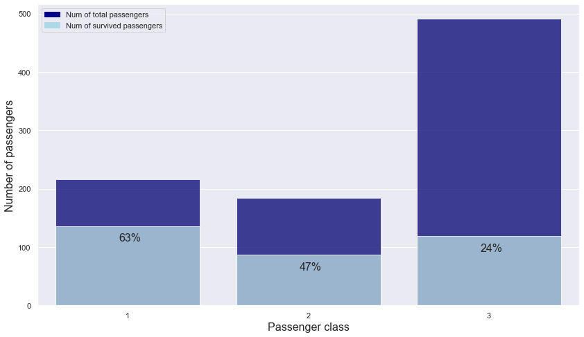
• As the class goes up one level, the chance of surviving increases by about 1.5 times.
  -> passenger class is important in predicting survival

ticket_number

np.sum(titanic["ticket_number"].isnull())

0

• There is no missing value in the ticket_number column

titanic.ticket_number

0             A/5 21171
1              PC 17599
2      STON/O2. 3101282
3                113803
4                373450
             ...       
886              211536
887              112053
888          W./C. 6607
889              111369
890              370376
Name: ticket_number, Length: 891, dtype: object

• Ticket numbers have a form of alphabet + number or just number.
  -> Let’s divide the ticket number into ticket_number_alphabet and ticket_number_number.

titanic.loc[titanic["ticket_number"].str.split(" ").str[1].isnull() == False, "ticket_number_alphabet"] = titanic[titanic["ticket_number"].str.split(" ").str[1].isnull() == False].ticket_number.str.split(" ").str[0]
titanic["ticket_number_alphabet"] = titanic.ticket_number_alphabet.fillna("non")

titanic.head()

	is_survived	p_class	name	sex	age	num_sb_sp	num_pr_ch	ticket_number	ticket_fare	cabin_number	embark_port	ticket_number_alphabet
0	0	3	Braund, Mr. Owen Harris	male	22.0	1	0	A/5 21171	7.2500	NaN	S	A/5
1	1	1	Cumings, Mrs. John Bradley (Florence Briggs Th...	female	38.0	1	0	PC 17599	71.2833	C85	C	PC
2	1	3	Heikkinen, Miss. Laina	female	26.0	0	0	STON/O2. 3101282	7.9250	NaN	S	STON/O2.
3	1	1	Futrelle, Mrs. Jacques Heath (Lily May Peel)	female	35.0	1	0	113803	53.1000	C123	S	non
4	0	3	Allen, Mr. William Henry	male	35.0	0	0	373450	8.0500	NaN	S	non

titanic.loc[titanic.ticket_number_alphabet == "non", "ticket_number_number"] = titanic[titanic.ticket_number_alphabet == "non"]["ticket_number"].str.split(" ").str[0]
titanic.loc[titanic.ticket_number_alphabet != "non", "ticket_number_number"] = titanic[titanic.ticket_number_alphabet != "non"]["ticket_number"].str.split(" ").str[1]
titanic.loc[titanic.ticket_number.str.split(" ").str[2].isnull() == False, "ticket_number_number"] = titanic[titanic.ticket_number.str.split(" ").str[2].isnull() == False].ticket_number.str.split(" ").str[2]

titanic[["ticket_number", "ticket_number_alphabet", "ticket_number_number"]]

	ticket_number	ticket_number_alphabet	ticket_number_number
0	A/5 21171	A/5	21171
1	PC 17599	PC	17599
2	STON/O2. 3101282	STON/O2.	3101282
3	113803	non	113803
4	373450	non	373450
...	...	...	...
886	211536	non	211536
887	112053	non	112053
888	W./C. 6607	W./C.	6607
889	111369	non	111369
890	370376	non	370376

891 rows × 3 columns

Aslo, if we sort the data by ticket number,

titanic.sort_values("ticket_number")

	is_survived	p_class	name	sex	age	num_sb_sp	num_pr_ch	ticket_number	ticket_fare	cabin_number	embark_port	ticket_number_alphabet	ticket_number_number
504	1	1	Maioni, Miss. Roberta	female	16.0	0	0	110152	86.500	B79	S	non	110152
257	1	1	Cherry, Miss. Gladys	female	30.0	0	0	110152	86.500	B77	S	non	110152
759	1	1	Rothes, the Countess. of (Lucy Noel Martha Dye...	female	33.0	0	0	110152	86.500	B77	S	non	110152
262	0	1	Taussig, Mr. Emil	male	52.0	1	1	110413	79.650	E67	S	non	110413
558	1	1	Taussig, Mrs. Emil (Tillie Mandelbaum)	female	39.0	1	1	110413	79.650	E67	S	non	110413
...	...	...	...	...	...	...	...	...	...	...	...	...	...
235	0	3	Harknett, Miss. Alice Phoebe	female	NaN	0	0	W./C. 6609	7.550	NaN	S	W./C.	6609
92	0	1	Chaffee, Mr. Herbert Fuller	male	46.0	1	0	W.E.P. 5734	61.175	E31	S	W.E.P.	5734
219	0	2	Harris, Mr. Walter	male	30.0	0	0	W/C 14208	10.500	NaN	S	W/C	14208
540	1	1	Crosby, Miss. Harriet R	female	36.0	0	2	WE/P 5735	71.000	B22	S	WE/P	5735
745	0	1	Crosby, Capt. Edward Gifford	male	70.0	1	1	WE/P 5735	71.000	B22	S	WE/P	5735

891 rows × 13 columns

• then it seems that rows that have the same ticket number have the same ticket fare. Let’s check this hypothesis for all rows.

merged_by_ticket_number = titanic.merge(titanic, on = "ticket_number", how = "left")
merged_by_ticket_number[merged_by_ticket_number.ticket_fare_x != merged_by_ticket_number.ticket_fare_y]

	is_survived_x	p_class_x	name_x	sex_x	age_x	num_sb_sp_x	num_pr_ch_x	ticket_number	ticket_fare_x	cabin_number_x	...	name_y	sex_y	age_y	num_sb_sp_y	num_pr_ch_y	ticket_fare_y	cabin_number_y	embark_port_y	ticket_number_alphabet_y	ticket_number_number_y
248	0	3	Osen, Mr. Olaf Elon	male	16.0	0	0	7534	9.2167	NaN	...	Gustafsson, Mr. Alfred Ossian	male	20.0	0	0	9.8458	NaN	S	non	7534
1570	0	3	Gustafsson, Mr. Alfred Ossian	male	20.0	0	0	7534	9.8458	NaN	...	Osen, Mr. Olaf Elon	male	16.0	0	0	9.2167	NaN	S	non	7534

2 rows × 25 columns

• There are only 2 people who have the same ticket number but have different ticket fares. So, I think this case is just an outlier, and we can think that if the ticket number is the same, then the ticket fare is also the same.

If we check some cases that have the same ticket number,

merged_by_ticket_number[["name_x", "name_y", "ticket_fare_x", "ticket_fare_y", "ticket_number"]].sort_values(["ticket_number", "name_x"]).head(20)

	name_x	name_y	ticket_fare_x	ticket_fare_y	ticket_number
460	Cherry, Miss. Gladys	Cherry, Miss. Gladys	86.50	86.50	110152
461	Cherry, Miss. Gladys	Maioni, Miss. Roberta	86.50	86.50	110152
462	Cherry, Miss. Gladys	Rothes, the Countess. of (Lucy Noel Martha Dye...	86.50	86.50	110152
889	Maioni, Miss. Roberta	Cherry, Miss. Gladys	86.50	86.50	110152
890	Maioni, Miss. Roberta	Maioni, Miss. Roberta	86.50	86.50	110152
891	Maioni, Miss. Roberta	Rothes, the Countess. of (Lucy Noel Martha Dye...	86.50	86.50	110152
1345	Rothes, the Countess. of (Lucy Noel Martha Dye...	Cherry, Miss. Gladys	86.50	86.50	110152
1346	Rothes, the Countess. of (Lucy Noel Martha Dye...	Maioni, Miss. Roberta	86.50	86.50	110152
1347	Rothes, the Countess. of (Lucy Noel Martha Dye...	Rothes, the Countess. of (Lucy Noel Martha Dye...	86.50	86.50	110152
1026	Taussig, Miss. Ruth	Taussig, Mr. Emil	79.65	79.65	110413
1027	Taussig, Miss. Ruth	Taussig, Mrs. Emil (Tillie Mandelbaum)	79.65	79.65	110413
1028	Taussig, Miss. Ruth	Taussig, Miss. Ruth	79.65	79.65	110413
473	Taussig, Mr. Emil	Taussig, Mr. Emil	79.65	79.65	110413
474	Taussig, Mr. Emil	Taussig, Mrs. Emil (Tillie Mandelbaum)	79.65	79.65	110413
475	Taussig, Mr. Emil	Taussig, Miss. Ruth	79.65	79.65	110413
987	Taussig, Mrs. Emil (Tillie Mandelbaum)	Taussig, Mr. Emil	79.65	79.65	110413
988	Taussig, Mrs. Emil (Tillie Mandelbaum)	Taussig, Mrs. Emil (Tillie Mandelbaum)	79.65	79.65	110413
989	Taussig, Mrs. Emil (Tillie Mandelbaum)	Taussig, Miss. Ruth	79.65	79.65	110413
842	Clifford, Mr. George Quincy	Porter, Mr. Walter Chamberlain	52.00	52.00	110465
843	Clifford, Mr. George Quincy	Clifford, Mr. George Quincy	52.00	52.00	110465

• then we can infer that peoples who have the same ticket number are companions who were traveling together. Since if companions are not family members, then this information is not in the num_sb_sp and num_pr_ch columns.
  -> let’s make a new column that shows how many companions were there for each passenger based on ticket number.

titanic = titanic.merge(titanic["ticket_number"].value_counts().reset_index().rename(columns = {"index" : "ticket_number", "ticket_number" : "num_cmp_by_ticket"}), \
                        on = "ticket_number", how = "left")
titanic["num_cmp_by_ticket"] = titanic["num_cmp_by_ticket"] - 1 # only one passenger with no companion has to have value 0
titanic.head()

	is_survived	p_class	name	sex	age	num_sb_sp	num_pr_ch	ticket_number	ticket_fare	cabin_number	embark_port	ticket_number_alphabet	ticket_number_number	num_cmp_by_ticket
0	0	3	Braund, Mr. Owen Harris	male	22.0	1	0	A/5 21171	7.2500	NaN	S	A/5	21171	0
1	1	1	Cumings, Mrs. John Bradley (Florence Briggs Th...	female	38.0	1	0	PC 17599	71.2833	C85	C	PC	17599	0
2	1	3	Heikkinen, Miss. Laina	female	26.0	0	0	STON/O2. 3101282	7.9250	NaN	S	STON/O2.	3101282	0
3	1	1	Futrelle, Mrs. Jacques Heath (Lily May Peel)	female	35.0	1	0	113803	53.1000	C123	S	non	113803	1
4	0	3	Allen, Mr. William Henry	male	35.0	0	0	373450	8.0500	NaN	S	non	373450	0

• But this can be different from the result from the sum of num_sb_sp and num_pr_ch.
  -> let’s cacluate num_cmp_by_sb_sp_pr_ch and compare this value to num_cmp_by_ticket.

titanic["num_cmp_by_sb_sp_pr_ch"] = titanic["num_sb_sp"] + titanic["num_pr_ch"]
titanic[titanic.num_cmp_by_ticket != titanic.num_cmp_by_sb_sp_pr_ch]

	is_survived	p_class	name	sex	age	num_sb_sp	num_pr_ch	ticket_number	ticket_fare	cabin_number	embark_port	ticket_number_alphabet	ticket_number_number	num_cmp_by_ticket	num_cmp_by_sb_sp_pr_ch
0	0	3	Braund, Mr. Owen Harris	male	22.0	1	0	A/5 21171	7.2500	NaN	S	A/5	21171	0	1
1	1	1	Cumings, Mrs. John Bradley (Florence Briggs Th...	female	38.0	1	0	PC 17599	71.2833	C85	C	PC	17599	0	1
7	0	3	Palsson, Master. Gosta Leonard	male	2.0	3	1	349909	21.0750	NaN	S	non	349909	3	4
10	1	3	Sandstrom, Miss. Marguerite Rut	female	4.0	1	1	PP 9549	16.7000	G6	S	PP	9549	1	2
16	0	3	Rice, Master. Eugene	male	2.0	4	1	382652	29.1250	NaN	Q	non	382652	4	5
...	...	...	...	...	...	...	...	...	...	...	...	...	...	...	...
866	1	2	Duran y More, Miss. Asuncion	female	27.0	1	0	SC/PARIS 2149	13.8583	NaN	C	SC/PARIS	2149	0	1
871	1	1	Beckwith, Mrs. Richard Leonard (Sallie Monypeny)	female	47.0	1	1	11751	52.5542	D35	S	non	11751	1	2
876	0	3	Gustafsson, Mr. Alfred Ossian	male	20.0	0	0	7534	9.8458	NaN	S	non	7534	1	0
885	0	3	Rice, Mrs. William (Margaret Norton)	female	39.0	0	5	382652	29.1250	NaN	Q	non	382652	4	5
888	0	3	Johnston, Miss. Catherine Helen "Carrie"	female	NaN	1	2	W./C. 6607	23.4500	NaN	S	W./C.	6607	1	3

288 rows × 15 columns

• There are 288 cases where the number of companions based on ticket number is different from the number of companions based on num_sb_sp and num_pr_ch.
  -> Let’s make num_cmp = max(num_cmp_by_ticket, num_cmp_by_sb_sp_pr_ch)

titanic["num_cmp"] = titanic[["num_cmp_by_ticket", "num_cmp_by_sb_sp_pr_ch"]].max(axis = 1)
titanic.drop(["num_cmp_by_ticket", "num_cmp_by_sb_sp_pr_ch"], axis = 1, inplace = True)

titanic.head()

	is_survived	p_class	name	sex	age	num_sb_sp	num_pr_ch	ticket_number	ticket_fare	cabin_number	embark_port	ticket_number_alphabet	ticket_number_number	num_cmp
0	0	3	Braund, Mr. Owen Harris	male	22.0	1	0	A/5 21171	7.2500	NaN	S	A/5	21171	1
1	1	1	Cumings, Mrs. John Bradley (Florence Briggs Th...	female	38.0	1	0	PC 17599	71.2833	C85	C	PC	17599	1
2	1	3	Heikkinen, Miss. Laina	female	26.0	0	0	STON/O2. 3101282	7.9250	NaN	S	STON/O2.	3101282	0
3	1	1	Futrelle, Mrs. Jacques Heath (Lily May Peel)	female	35.0	1	0	113803	53.1000	C123	S	non	113803	1
4	0	3	Allen, Mr. William Henry	male	35.0	0	0	373450	8.0500	NaN	S	non	373450	0

titanic.shape

(891, 14)

ticket_number_alphabet

len(titanic.ticket_number_alphabet.unique())

43

titanic.ticket_number_alphabet.value_counts()

non           665
PC             60
C.A.           27
STON/O         12
A/5            10
W./C.           9
CA.             8
SOTON/O.Q.      8
SOTON/OQ        7
A/5.            7
CA              6
STON/O2.        6
C               5
F.C.C.          5
S.O.C.          5
SC/PARIS        5
SC/Paris        4
S.O./P.P.       3
PP              3
A/4.            3
A/4             3
SC/AH           3
A./5.           2
SOTON/O2        2
A.5.            2
WE/P            2
S.C./PARIS      2
P/PP            2
F.C.            1
SC              1
S.W./PP         1
A/S             1
Fa              1
SCO/W           1
SW/PP           1
W/C             1
S.C./A.4.       1
S.O.P.          1
A4.             1
W.E.P.          1
SO/C            1
S.P.            1
C.A./SOTON      1
Name: ticket_number_alphabet, dtype: int64

• There are 42 distinct kinds of prefixes in the ticket number, and almost ticket numbers don’t have a prefix alphabet. But it is hard to interpret the ticket number alphabet or to find some relationship with other columns.
  -> Do not use ticket_number_alphabet

**ticket_number_number ~ p_class

is_survived**

Let’s check if there is a relationship between ticket_number_number and p_class

plt.figure(figsize = (14, 8))
sns.boxplot(data = pd.concat([titanic.p_class, titanic[titanic.ticket_number_number != "LINE"].ticket_number_number.astype("int32")], axis = 1), x = "p_class", y = "ticket_number_number")
plt.xlabel("Passenger class", fontsize = 14)
plt.ylabel("Ticket number part", fontsize = 14)
plt.show()

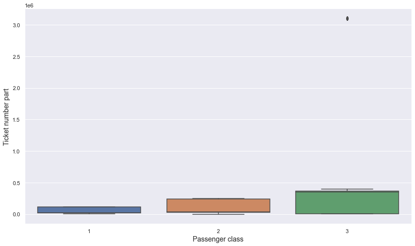
• It is hard to find relationship between ticket_number_number and p_class.

Let’s check if there is a relationship between ticket_number_number and is_survived

plt.figure(figsize = (14, 8))
sns.boxplot(data = pd.concat([titanic.is_survived, titanic[titanic.ticket_number_number != "LINE"].ticket_number_number.astype("int32")], axis = 1), x = "is_survived", y = "ticket_number_number")
plt.xlabel("Is survived", fontsize = 14)
plt.ylabel("Ticket number part", fontsize = 14)
plt.show()

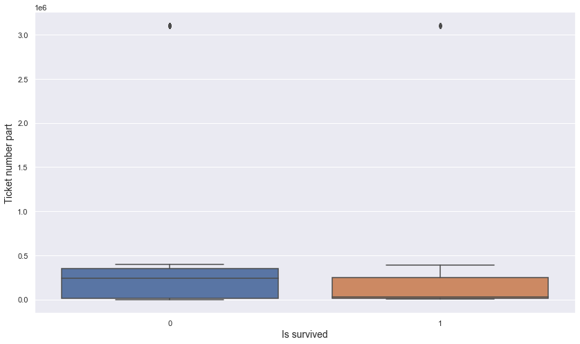
• It is hard to find relationship between ticket_number_number and p_class.
  -> Do not use the ticket_number_number

ticket_fare

np.sum(titanic["ticket_fare"].isnull())

0

• There is no missing value in the ticket_fare column

titanic["ticket_fare"].describe()

count    891.000000
mean      32.204208
std       49.693429
min        0.000000
25%        7.910400
50%       14.454200
75%       31.000000
max      512.329200
Name: ticket_fare, dtype: float64

plt.figure(figsize = (14, 8))

sns.histplot(titanic.ticket_fare)
plt.xlabel("Ticket fare", fontsize = 14)
plt.ylabel("Count", fontsize = 14)
plt.show()

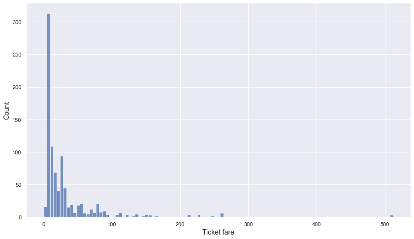
• Minimum value is 0 and maximum value is 512.33.
• 75% of ticket fares are under 31.
• These numerical values and the histogram show that the standard deviation is very large.
  -> Let’s check the histogram of ticket fares under the 95% percentile.

ticket_fares_95 = np.percentile(titanic["ticket_fare"], 95)
ticket_fares_95

112.07915

fig, (ax_box, ax_hist) = plt.subplots(2, sharex = True, gridspec_kw = {"height_ratios": (.2, .8)}, figsize = (10, 7))

sns.boxplot(x = titanic.ticket_fare, ax = ax_box, showfliers = False)
sns.histplot(x = titanic[titanic["ticket_fare"] <= ticket_fares_95].ticket_fare, ax = ax_hist)

plt.xlabel("Ticket Fare", fontsize = 16)
plt.ylabel("Count", fontsize = 16)
ax_box.set_xlabel("")

plt.show()

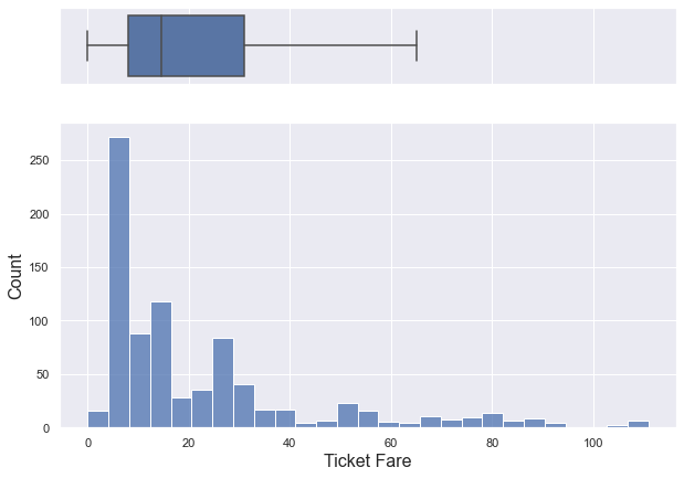
• 50% of ticket fares are under 14 and almost ticket fares are under 30.

Now, let’s check outliers

titanic[titanic["ticket_fare"] == 0]

	is_survived	p_class	name	sex	age	num_sb_sp	num_pr_ch	ticket_number	ticket_fare	cabin_number	embark_port	ticket_number_alphabet	ticket_number_number	num_cmp
179	0	3	Leonard, Mr. Lionel	male	36.0	0	0	LINE	0.0	NaN	S	non	LINE	3
263	0	1	Harrison, Mr. William	male	40.0	0	0	112059	0.0	B94	S	non	112059	0
271	1	3	Tornquist, Mr. William Henry	male	25.0	0	0	LINE	0.0	NaN	S	non	LINE	3
277	0	2	Parkes, Mr. Francis "Frank"	male	NaN	0	0	239853	0.0	NaN	S	non	239853	2
302	0	3	Johnson, Mr. William Cahoone Jr	male	19.0	0	0	LINE	0.0	NaN	S	non	LINE	3
413	0	2	Cunningham, Mr. Alfred Fleming	male	NaN	0	0	239853	0.0	NaN	S	non	239853	2
466	0	2	Campbell, Mr. William	male	NaN	0	0	239853	0.0	NaN	S	non	239853	2
481	0	2	Frost, Mr. Anthony Wood "Archie"	male	NaN	0	0	239854	0.0	NaN	S	non	239854	0
597	0	3	Johnson, Mr. Alfred	male	49.0	0	0	LINE	0.0	NaN	S	non	LINE	3
633	0	1	Parr, Mr. William Henry Marsh	male	NaN	0	0	112052	0.0	NaN	S	non	112052	0
674	0	2	Watson, Mr. Ennis Hastings	male	NaN	0	0	239856	0.0	NaN	S	non	239856	0
732	0	2	Knight, Mr. Robert J	male	NaN	0	0	239855	0.0	NaN	S	non	239855	0
806	0	1	Andrews, Mr. Thomas Jr	male	39.0	0	0	112050	0.0	A36	S	non	112050	0
815	0	1	Fry, Mr. Richard	male	NaN	0	0	112058	0.0	B102	S	non	112058	0
822	0	1	Reuchlin, Jonkheer. John George	male	38.0	0	0	19972	0.0	NaN	S	non	19972	0

• There are only 15 rows whose ticket fare is 0.0. So 0 may mean a missing value.
  -> In the above ticket_number EDA, we have found that the same ticket numbers have the same ticket fares. So let’s check if other rows have non-zero fare with the same ticket numbers as the above table.

for tn in titanic[titanic["ticket_fare"] == 0].ticket_number.unique():
    print(tn, " :", titanic[(titanic["ticket_fare"] != 0) & (titanic.ticket_number == tn)].shape)

LINE  : (0, 14)
112059  : (0, 14)
239853  : (0, 14)
239854  : (0, 14)
112052  : (0, 14)
239856  : (0, 14)
239855  : (0, 14)
112050  : (0, 14)
112058  : (0, 14)
19972  : (0, 14)

• All row whose fare is 0 doesn’t have other rows that have the same ticket number as the non-zero fare. So it isn’t possible to impute the ticket fare values with ticket number information.
  -> Since there are no missing values in p_class, let’s use p_class to impute the missing value in the ticket_fare column.

ticket_fare ~ p_class

Let’s check relationship between ticket_fare and p_class

titanic.groupby("p_class").ticket_fare.median().reset_index().rename({"ticket_fare" : "ticket_fare_median"}, axis = 1) \
    .merge(titanic.groupby("p_class").ticket_fare.mean().reset_index().rename({"ticket_fare" : "ticket_fare_mean"}, axis = 1), on = "p_class", how = "left")

	p_class	ticket_fare_median	ticket_fare_mean
0	1	60.2875	84.154687
1	2	14.2500	20.662183
2	3	8.0500	13.675550

plt.figure(figsize = (14, 8))

sns.boxplot(data = titanic, x = "p_class", y = "ticket_fare")
plt.xlabel("Passenger class", fontsize = 14)
plt.ylabel("Ticket fare", fontsize = 14)
plt.show()

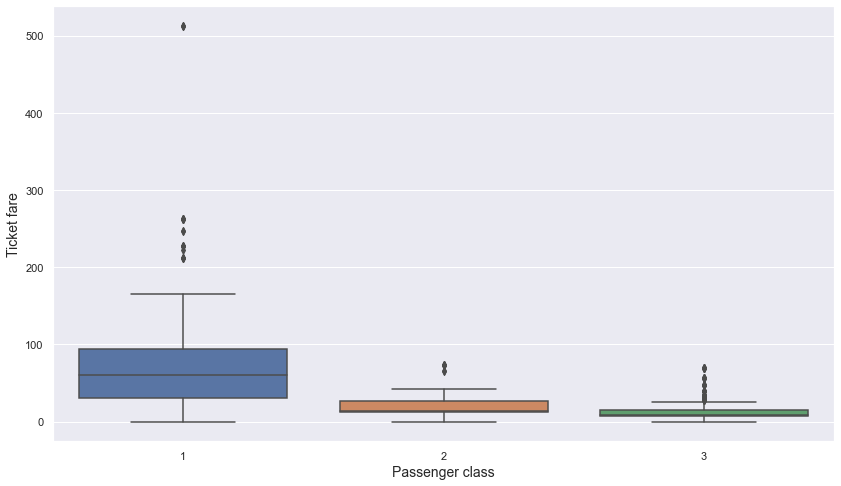
• We can see that there are meaningful differences in mean and median values of ticket fares between passenger classes.
  -> Since there were no missing values in passenger class, I think it is a good way to impute missing value in ticket fare with the mean or median value of each passenger class. In the above box plot, we can see that there are some extreme values in passenger class = 1. Since mean is affected a lot with extreme values, let’s use median instead of mean to impute ticket fare.

p_class_fare_median = titanic.groupby("p_class").ticket_fare.median().reset_index().rename({"ticket_fare" : "ticket_fare_median"}, axis = 1)
p_class_fare_median

	p_class	ticket_fare_median
0	1	60.2875
1	2	14.2500
2	3	8.0500

titanic.loc[(titanic.ticket_fare == 0) & (titanic.p_class == 1), "ticket_fare"] = p_class_fare_median[p_class_fare_median.p_class == 1].ticket_fare_median.values[0]
titanic.loc[(titanic.ticket_fare == 0) & (titanic.p_class == 2), "ticket_fare"] = p_class_fare_median[p_class_fare_median.p_class == 2].ticket_fare_median.values[0]
titanic.loc[(titanic.ticket_fare == 0) & (titanic.p_class == 3), "ticket_fare"] = p_class_fare_median[p_class_fare_median.p_class == 3].ticket_fare_median.values[0]

titanic.shape

(891, 14)

titanic[titanic.ticket_fare == 0]

	is_survived	p_class	name	sex	age	num_sb_sp	num_pr_ch	ticket_number	ticket_fare	cabin_number	embark_port	ticket_number_alphabet	ticket_number_number	num_cmp

titanic[titanic.ticket_fare.isnull()]

	is_survived	p_class	name	sex	age	num_sb_sp	num_pr_ch	ticket_number	ticket_fare	cabin_number	embark_port	ticket_number_alphabet	ticket_number_number	num_cmp

ticket_fare ~ is_survived

plt.figure(figsize = (14, 8))

sns.boxplot(data = titanic, x = "is_survived", y = "ticket_fare", showfliers = False)
plt.xlabel("Is survived", fontsize = 14)
plt.ylabel("Ticket fare", fontsize = 14)
plt.show()

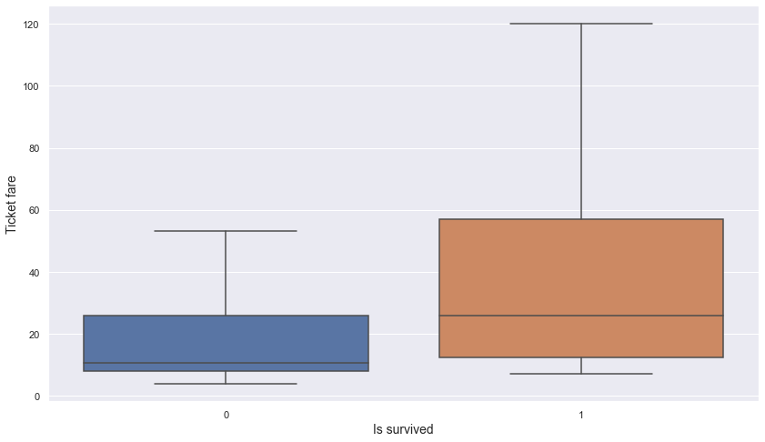
• It seems that passengers who paid the higher fare may have been more likely to have survived.
  -> Let’s cut the ticket_fare into 3 categories and compare the survival rate of each category.

titanic['ticket_fare_category'] = pd.qcut(titanic.ticket_fare, 3)
titanic.ticket_fare_category.value_counts()

(8.676, 26.25]                300
(4.010999999999999, 8.676]    297
(26.25, 512.329]              294
Name: ticket_fare_category, dtype: int64

ticket_fare_category_is_survived = pd.pivot_table(index = "ticket_fare_category", columns = "is_survived", aggfunc = len, fill_value = 0, data = titanic[["ticket_fare_category", "is_survived"]])
ticket_fare_category_is_survived = ticket_fare_category_is_survived.reset_index().rename_axis(None, axis = 1)
ticket_fare_category_is_survived["total"] = ticket_fare_category_is_survived[0] + ticket_fare_category_is_survived[1]
ticket_fare_category_is_survived["ratio"] = np.round(ticket_fare_category_is_survived[1] / ticket_fare_category_is_survived.total, 2)
ticket_fare_category_is_survived

	ticket_fare_category	0	1	total	ratio
0	(4.010999999999999, 8.676]	236	61	297	0.21
1	(8.676, 26.25]	180	120	300	0.40
2	(26.25, 512.329]	133	161	294	0.55

plt.figure(figsize = (14, 8))

# bar graph for total students
color = "darkblue"
ax1 = sns.barplot(x = "ticket_fare_category", y = "total", color = color, alpha = 0.8, \
                  data = ticket_fare_category_is_survived)
top_bar = mpatches.Patch(color = color, label = 'Num of total passengers')

# bar graph for students have research experience
color = "lightblue"
ax2 = sns.barplot(x = "ticket_fare_category", y = 1,  color = color, alpha = 0.8, \
                  data = ticket_fare_category_is_survived)
ax2.set_xlabel("Ticket fare category", fontsize = 16)
ax2.set_ylabel("Number of passengers", fontsize = 16)
low_bar = mpatches.Patch(color = color, label = 'Num of survived passengers')

# ratio
plt.text(s = "20%", x = -0.05, y = 35, fontsize = 16)
plt.text(s = "41%", x = 0.95, y = 95, fontsize = 16)
plt.text(s = "56%", x = 1.95, y = 136, fontsize = 16)

plt.legend(handles=[top_bar, low_bar])
plt.show()

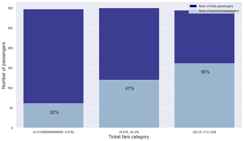
• It can be seen that the category that paid a higher fare showed a higher survival rate.
  -> Use the ticket_fare_category column.

cabin_number

titanic["cabin_number"]

0       NaN
1       C85
2       NaN
3      C123
4       NaN
       ... 
886     NaN
887     B42
888     NaN
889    C148
890     NaN
Name: cabin_number, Length: 891, dtype: object

• cabin_number is form of alphabet + number
  -> Let’s divide the alphabet part and make this alphabet as a new column

titanic["cabin_alphabet"] = titanic.cabin_number.str[0]
titanic["cabin_alphabet"] = titanic["cabin_alphabet"].fillna("n")

titanic.cabin_alphabet.value_counts()

n    687
C     59
B     47
D     33
E     32
A     15
F     13
G      4
T      1
Name: cabin_alphabet, dtype: int64

• n means missing values. There are too many missing values in the cabin_alphabet column
  -> If it is not related with is_survived or p_class, then do not use cabin_number and cabin_alphabet

**cabin_alphabet ~ is_survived

p_class**

Let’s check relationship between cabin_alphabet and p_class

pt = pd.pivot_table(index = "p_class", columns = "cabin_alphabet", aggfunc = len, fill_value = 0, data = titanic[["p_class", "cabin_alphabet"]])
pt

cabin_alphabet	A	B	C	D	E	F	G	T	n
p_class
1	15	47	59	29	25	0	0	1	40
2	0	0	0	4	4	8	0	0	168
3	0	0	0	0	3	5	4	0	479

• There are too many missing values in passenger class = 2 and passenger class = 3

Let’s check relationship between cabin_alphabet and is_survived.

pt = pd.pivot_table(index = "is_survived", columns = "cabin_alphabet", aggfunc = len, fill_value = 0, data = titanic[["is_survived", "cabin_alphabet"]])
pt

cabin_alphabet	A	B	C	D	E	F	G	T	n
is_survived
0	8	12	24	8	8	5	2	1	481
1	7	35	35	25	24	8	2	0	206

• Also, there are too many missing values in both is_survived cases
  -> Do not use cabin_number and cabin_alphabet

embark_port

titanic.embark_port.value_counts().reset_index().rename(columns = {"index" : "embark_port", "embark_port" : "count"})

	embark_port	count
0	S	644
1	C	168
2	Q	77

plt.figure(figsize = (14, 8))
sns.barplot(data = titanic.embark_port.value_counts().reset_index().rename(columns = {"index" : "embark_port", "embark_port" : "count"}),
            x = "embark_port",
            y = "count")
plt.xlabel("Embark port", fontsize = 14)
plt.ylabel("Count", fontsize = 14)
plt.show()

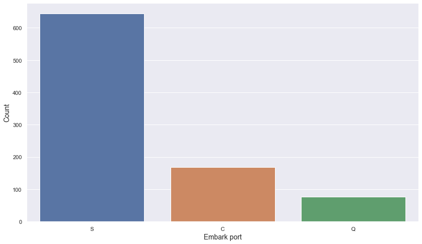
• Most passengers boarded from Southampton (S) port
• Least passengers boarded from Queenstown (Q) port

titanic[titanic.embark_port.isnull()]

	is_survived	p_class	name	sex	age	num_sb_sp	num_pr_ch	ticket_number	ticket_fare	cabin_number	embark_port	ticket_number_alphabet	ticket_number_number	num_cmp	ticket_fare_category	cabin_alphabet
61	1	1	Icard, Miss. Amelie	female	38.0	0	0	113572	80.0	B28	NaN	non	113572	1	(26.25, 512.329]	B
829	1	1	Stone, Mrs. George Nelson (Martha Evelyn)	female	62.0	0	0	113572	80.0	B28	NaN	non	113572	1	(26.25, 512.329]	B

• There are only 2 rows where embark_port has a missing value.
  -> Fill missing value with the most common embarked_pork value: S

titanic["embark_port"] = titanic["embark_port"].fillna("S")

np.sum(titanic.embark_port.isnull())

0

embark_port ~ p_class

Let’s check a relationship between embark_port and p_class

pd.pivot_table(index = "p_class", columns = "embark_port", aggfunc = len, fill_value = 0, data = titanic[titanic.ticket_fare != 0][["p_class", "embark_port"]])

embark_port	C	Q	S
p_class
1	85	2	129
2	17	3	164
3	66	72	353

• Almost every people who boarded from Q was 3 passenger class.
  -> Since embark_port has some influence in passenger class, let’s check the relationship between embark_port and is_survived

embark_port ~ is_survived

embark_port_is_survived = titanic.groupby(["embark_port","is_survived"]).count().name.unstack().reset_index()
embark_port_is_survived = embark_port_is_survived.rename_axis(None, axis = 1)
embark_port_is_survived["total"] = embark_port_is_survived[0] + embark_port_is_survived[1]
embark_port_is_survived["ratio"] = np.round(embark_port_is_survived[1] / embark_port_is_survived.total, 2)
embark_port_is_survived

	embark_port	0	1	total	ratio
0	C	75	93	168	0.55
1	Q	47	30	77	0.39
2	S	427	219	646	0.34

plt.figure(figsize = (14, 8))

# bar graph for total students
color = "darkblue"
ax1 = sns.barplot(x = "embark_port", y = "total", color = color, alpha = 0.8, \
                  data = embark_port_is_survived)
top_bar = mpatches.Patch(color = color, label = 'Num of total passengers')

# bar graph for students have research experience
color = "lightblue"
ax2 = sns.barplot(x = "embark_port", y = 1,  color = color, alpha = 0.8, \
                  data = embark_port_is_survived)
ax2.set_xlabel("Port of Embarkation", fontsize = 16)
ax2.set_ylabel("Number of passengers", fontsize = 16)
low_bar = mpatches.Patch(color = color, label = 'Num of survived passengers')

# ratio
plt.text(s = "55%", x = -0.05, y = 68, fontsize = 16)
plt.text(s = "39%", x = 0.95, y = 5, fontsize = 16)
plt.text(s = "34%", x = 1.95, y = 194, fontsize = 16)

plt.legend(handles=[top_bar, low_bar])
plt.show()

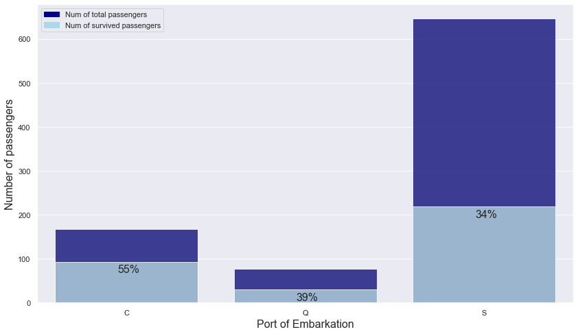
• People boarded from Q and S have similar survival rates: about 39% and 34%.
• People boarded from C have a higher survival rate than people boarded from other ports.
  -> Use embark_port column

1.1. Person related columns: name, sex, age

name

np.sum(titanic.name.isnull())

0

• There is no missing value in the name column.

len(titanic.name.unique())

891

• All 891 rows have differnt name values.
  -> Let’s think about more general features from name.

titanic.name.head(10)

0                              Braund, Mr. Owen Harris
1    Cumings, Mrs. John Bradley (Florence Briggs Th...
2                               Heikkinen, Miss. Laina
3         Futrelle, Mrs. Jacques Heath (Lily May Peel)
4                             Allen, Mr. William Henry
5                                     Moran, Mr. James
6                              McCarthy, Mr. Timothy J
7                       Palsson, Master. Gosta Leonard
8    Johnson, Mrs. Oscar W (Elisabeth Vilhelmina Berg)
9                  Nasser, Mrs. Nicholas (Adele Achem)
Name: name, dtype: object

• We can see that names are a form of Last name + title + first name.
  -> Let’s extract the title from the name

titanic["name_title"] = titanic.name.str.extract(' ([A-Za-z]+)\.', expand=False)
titanic.name_title.value_counts()

Mr          517
Miss        182
Mrs         125
Master       40
Dr            7
Rev           6
Mlle          2
Major         2
Col           2
Countess      1
Capt          1
Ms            1
Sir           1
Lady          1
Mme           1
Don           1
Jonkheer      1
Name: name_title, dtype: int64

• There are too many uncommon titles that appear only a few times.
  -> Let’s replace uncommon titles.

titanic['name_title'] = titanic['name_title'].replace(['Lady', 'Countess','Capt', 'Col', 'Don', 'Dr', 'Major', \
                                                       'Rev', 'Sir', 'Jonkheer', 'Dona'], 'uncommon')

titanic['name_title'] = titanic['name_title'].replace('Mlle', 'Miss')
titanic['name_title'] = titanic['name_title'].replace('Ms', 'Miss')
titanic['name_title'] = titanic['name_title'].replace('Mme', 'Mrs')

titanic.name_title.value_counts()

Mr          517
Miss        185
Mrs         126
Master       40
uncommon     23
Name: name_title, dtype: int64

name_title ~ is_survived

Let’s check the relationship between name_title and is_survived.

name_title_is_survived = titanic.groupby(["name_title","is_survived"]).count().name.unstack().reset_index()
name_title_is_survived = name_title_is_survived.rename_axis(None, axis = 1)
name_title_is_survived["total"] = name_title_is_survived[0] + name_title_is_survived[1]
name_title_is_survived["ratio"] = np.round(name_title_is_survived[1] / name_title_is_survived.total, 2)
name_title_is_survived

	name_title	0	1	total	ratio
0	Master	17	23	40	0.57
1	Miss	55	130	185	0.70
2	Mr	436	81	517	0.16
3	Mrs	26	100	126	0.79
4	uncommon	15	8	23	0.35

plt.figure(figsize = (14, 8))

# bar graph for total students
color = "darkblue"
ax1 = sns.barplot(x = "name_title", y = "total", color = color, alpha = 0.8, \
                  data = name_title_is_survived)
top_bar = mpatches.Patch(color = color, label = 'Num of total passengers')

# bar graph for students have research experience
color = "lightblue"
ax2 = sns.barplot(x = "name_title", y = 1,  color = color, alpha = 0.8, \
                  data = name_title_is_survived)
ax2.set_xlabel("Name title", fontsize = 16)
ax2.set_ylabel("Number of passengers", fontsize = 16)
low_bar = mpatches.Patch(color = color, label = 'Num of survived passengers')

# ratio
for n in name_title_is_survived.index:
    plt.text(s = f"{np.round(name_title_is_survived.loc[n].ratio * 100, 2)} %", x = n - 0.1, y = name_title_is_survived.loc[n][1] + 5, color = "white")
 
    
plt.legend(handles=[top_bar, low_bar])
plt.show()

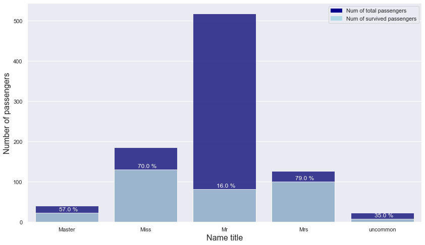
• Passengers with Miss and Mrs titles showed an overwhelming survival rate of over 70%
  -> Use name_title instead of name

sex

np.sum(titanic.sex.isnull())

0

• There is no missing value in the sex column.

titanic.sex.value_counts()

male      577
female    314
Name: sex, dtype: int64

plt.figure(figsize = (14, 8))
sns.barplot(data = titanic.sex.value_counts().reset_index().rename(columns = {"index" : "sex", "sex" : "count"}),
            x = "sex",
            y = "count")
plt.xlabel("Sex", fontsize = 14)
plt.ylabel("Count", fontsize = 14)
plt.show()

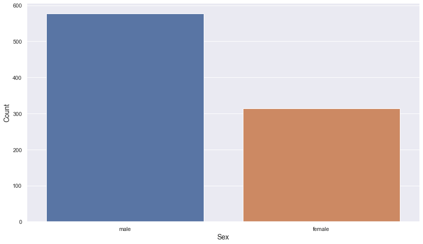
• There are about twice as many male passengers as female passengers.

sex ~ p_class

Let’s check the relationship between sex and p_class.

sex_p_class = pd.pivot_table(index = "p_class", columns = "sex", aggfunc = len, fill_value = 0, data = titanic[["p_class", "sex"]])
sex_p_class = sex_p_class.reset_index().rename_axis(None, axis = 1)
sex_p_class["total"] = sex_p_class["female"] + sex_p_class["male"]
sex_p_class["ratio"] = np.round(sex_p_class["male"] / sex_p_class.total, 2)
sex_p_class

	p_class	female	male	total	ratio
0	1	94	122	216	0.56
1	2	76	108	184	0.59
2	3	144	347	491	0.71

plt.figure(figsize = (14, 8))

# bar graph for total students
color = "darkblue"
ax1 = sns.barplot(x = "p_class", y = "total", color = color, alpha = 0.8, \
                  data = sex_p_class)
top_bar = mpatches.Patch(color = color, label = 'Num of total passengers')

# bar graph for students have research experience
color = "lightblue"
ax2 = sns.barplot(x = "p_class", y = "male",  color = color, alpha = 0.8, \
                  data = sex_p_class)
ax2.set_xlabel("Passenger class", fontsize = 16)
ax2.set_ylabel("Number of passengers", fontsize = 16)
low_bar = mpatches.Patch(color = color, label = 'Num of male passengers')

# ratio
plt.text(s = "56%", x = -0.05, y = 97, fontsize = 16)
plt.text(s = "59%", x = 0.95, y = 83, fontsize = 16)
plt.text(s = "71%", x = 1.95, y = 322, fontsize = 16)

plt.legend(handles=[top_bar, low_bar])
plt.show()

• Passengers from classes 1 and 2 have a similar male rate: about 56% and 59%
• Passengers from class 3 have a higher male rate than passengers from other classes.

sex ~ is_survived

sex_is_survived = pd.pivot_table(index = "sex", columns = "is_survived", aggfunc = len, fill_value = 0, data = titanic[["is_survived", "sex"]])
sex_is_survived = sex_is_survived.reset_index().rename_axis(None, axis = 1)
sex_is_survived["total"] = sex_is_survived[0] + sex_is_survived[1]
sex_is_survived["ratio"] = np.round(sex_is_survived[1] / sex_is_survived.total, 2)
sex_is_survived

	sex	0	1	total	ratio
0	female	81	233	314	0.74
1	male	468	109	577	0.19

plt.figure(figsize = (14, 8))

# bar graph for total students
color = "darkblue"
ax1 = sns.barplot(x = "sex", y = "total", color = color, alpha = 0.8, \
                  data = sex_is_survived)
top_bar = mpatches.Patch(color = color, label = 'Num of total passengers')

# bar graph for students have research experience
color = "lightblue"
ax2 = sns.barplot(x = "sex", y = 1,  color = color, alpha = 0.8, \
                  data = sex_is_survived)
ax2.set_xlabel("Sex", fontsize = 16)
ax2.set_ylabel("Number of passengers", fontsize = 16)
low_bar = mpatches.Patch(color = color, label = 'Num of survived passengers')

# ratio
plt.text(s = "74%", x = -0.05, y = 208, fontsize = 16)
plt.text(s = "19%", x = 0.95, y = 84, fontsize = 16)

plt.legend(handles=[top_bar, low_bar])
plt.show()

• We can see that sex had a huge impact on survival. Only 19% of the male passengers survived, while 74% of the female passengers survived.
  -> Use sex column

age

np.sum(titanic.age.isnull())

177

• There are 177 missing values in the age column
  -> Need to think about how to impute missing values.

titanic.age.describe()

count    714.000000
mean      29.699118
std       14.526497
min        0.420000
25%       20.125000
50%       28.000000
75%       38.000000
max       80.000000
Name: age, dtype: float64

fig, (ax_box, ax_hist) = plt.subplots(2, sharex = True, gridspec_kw = {"height_ratios": (.2, .8)}, figsize = (10, 7))

sns.boxplot(x = titanic.age, ax = ax_box, showfliers = False)
sns.histplot(x = titanic.age, ax = ax_hist)

plt.xlabel("Age", fontsize = 16)
plt.ylabel("Count", fontsize = 16)
ax_box.set_xlabel("")

plt.show()

• age shows a slightly bell-shaped distribution

For further analysis, let’s make new column of age category.

import math

math.log(0.04 * 0.05 * 0.06) * -2

18.056037630364457

math.log(0.6 * 0.25 * 0.01) * -2

13.004580341747944

titanic["age_category"] = pd.cut(titanic.age, 10)
titanic.age_category.value_counts()

(16.336, 24.294]    177
(24.294, 32.252]    169
(32.252, 40.21]     118
(40.21, 48.168]      70
(0.34, 8.378]        54
(8.378, 16.336]      46
(48.168, 56.126]     45
(56.126, 64.084]     24
(64.084, 72.042]      9
(72.042, 80.0]        2
Name: age_category, dtype: int64

**p_class ~ age

age_category**

Let’s check the relationship between p_class and age.

plt.figure(figsize = (14, 8))

sns.boxplot(data = titanic, x = "p_class", y = "age")
plt.xlabel("Passenger class", fontsize = 14)
plt.ylabel("Age", fontsize = 14)
plt.show()

• The better the class, the older the passengers in it tend to be.

Let’s see the relationship of passenger class and age by age category.

pt = pd.pivot_table(index = "p_class", columns = "age_category", aggfunc = len, fill_value = 0, data = titanic[["p_class", "age_category"]])

plt.figure(figsize = (14, 8))
sns.heatmap(pt, annot = True, cmap = 'BrBG');
plt.xlabel("Age category", fontsize = 14)
plt.ylabel("Passenger class", fontsize = 14)
plt.show()

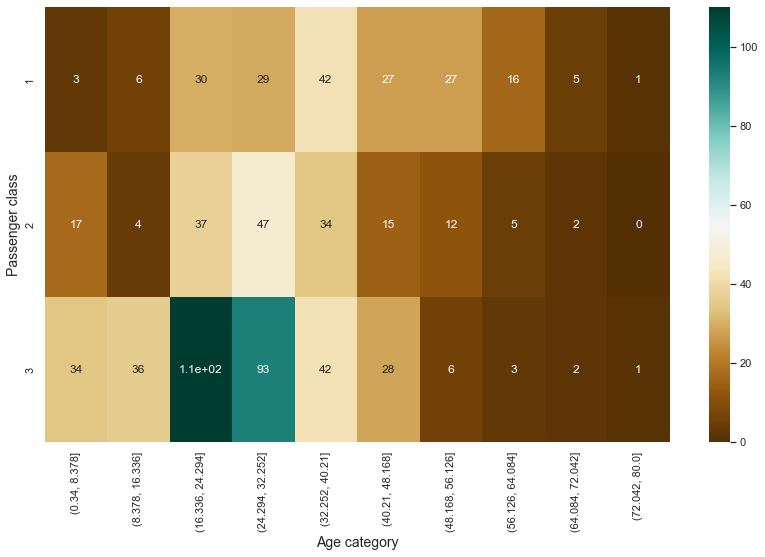
• In particular, in class 3, it can be seen that the proportion of young people is high.
• In classes 1 and 2, the proportion of passengers in the middle age group is high.
  -> There seems to be some relationship between age and class. So, let’s look at the relationship between age and survival rate.

**is_survived ~ age

age_category**

Let’s check the relationship between is_survived and age.

plt.figure(figsize = (14, 8))

sns.boxplot(data = titanic, x = "is_survived", y = "age")
plt.xlabel("Is survived", fontsize = 14)
plt.ylabel("Age", fontsize = 14)
plt.show()

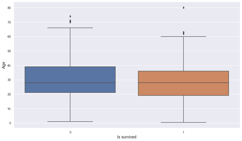
• There appears to be no difference in the distribution of age between the survived and non-survived groups.

age_category_is_survived = pd.pivot_table(index = "age_category", columns = "is_survived", aggfunc = len, fill_value = 0, data = titanic[["is_survived", "age_category"]])
age_category_is_survived = age_category_is_survived.reset_index().rename_axis(None, axis = 1)
age_category_is_survived["total"] = age_category_is_survived[0] + age_category_is_survived[1]
age_category_is_survived["ratio"] = np.round(age_category_is_survived[1] / age_category_is_survived.total, 2)
age_category_is_survived

	age_category	0	1	total	ratio
0	(0.34, 8.378]	18	36	54	0.67
1	(8.378, 16.336]	27	19	46	0.41
2	(16.336, 24.294]	114	63	177	0.36
3	(24.294, 32.252]	104	65	169	0.38
4	(32.252, 40.21]	66	52	118	0.44
5	(40.21, 48.168]	46	24	70	0.34
6	(48.168, 56.126]	24	21	45	0.47
7	(56.126, 64.084]	15	9	24	0.38
8	(64.084, 72.042]	9	0	9	0.00
9	(72.042, 80.0]	1	1	2	0.50

plt.figure(figsize = (14, 8))

# bar graph for total students
color = "darkblue"
ax1 = sns.barplot(x = "age_category", y = "total", color = color, alpha = 0.8, \
                  data = age_category_is_survived)
top_bar = mpatches.Patch(color = color, label = 'Num of total passengers')

# bar graph for students have research experience
color = "lightblue"
ax2 = sns.barplot(x = "age_category", y = 1,  color = color, alpha = 0.8, \
                  data = age_category_is_survived)
ax2.set_xlabel("Age category", fontsize = 16)
ax2.set_ylabel("Number of passengers", fontsize = 16)
low_bar = mpatches.Patch(color = color, label = 'Num of survived passengers')

# ratio
for n in age_category_is_survived.index:
    plt.text(s = f"{age_category_is_survived.loc[n].ratio * 100} %", x = n - 0.2, y = age_category_is_survived.loc[n][1] + 5, color = "lightblue")
 
    
plt.legend(handles=[top_bar, low_bar])
plt.show()

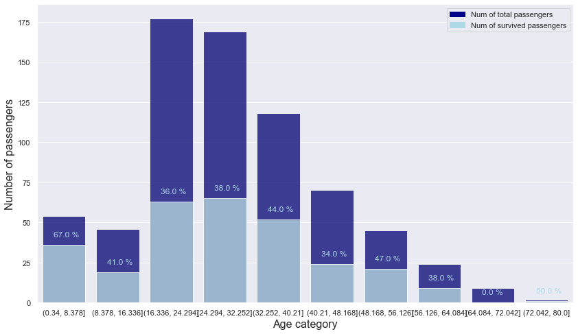
• It can be seen that the survival rate decreases with increasing age and then rises again.
  -> Use age category and age. Then since age has 177 missing values, we have to consider how to impute missing values in age.

age ~ sex

Let’s check the relationship between age and sex.

plt.figure(figsize = (14, 8))

sns.boxplot(data = titanic, x = "sex", y = "age")
plt.xlabel("Sex", fontsize = 14)
plt.ylabel("Age", fontsize = 14)
plt.show()

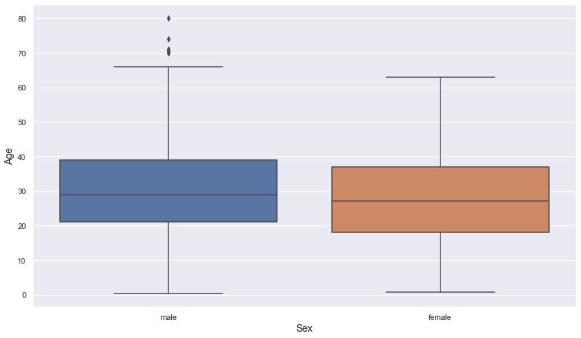
• There appears to be no difference in the distribution of age between the male and female groups.

Let’s check the distribution in more detail using age category.

age_sex = titanic.groupby(["age_category"]).sex.value_counts().unstack().fillna(0)
age_sex = age_sex.reset_index().rename_axis(None, axis = 1)
age_sex

	age_category	female	male
0	(0.34, 8.378]	26.0	28.0
1	(8.378, 16.336]	23.0	23.0
2	(16.336, 24.294]	68.0	109.0
3	(24.294, 32.252]	52.0	117.0
4	(32.252, 40.21]	44.0	74.0
5	(40.21, 48.168]	24.0	46.0
6	(48.168, 56.126]	16.0	29.0
7	(56.126, 64.084]	8.0	16.0
8	(64.084, 72.042]	0.0	9.0
9	(72.042, 80.0]	0.0	2.0

#define plot parameters
fig, axes = plt.subplots(ncols=2, sharey=True, figsize=(20, 8))

#specify background color and plot title
#fig.patch.set_facecolor('xkcd:light grey')
plt.figtext(.5,.9,"Population Pyramid ", fontsize=16, ha='center')
    
#define male and female bars
axes[0].barh(range(0, len(age_sex)), age_sex.male, align='center', color='darkblue')
axes[0].set(title='Males')
axes[1].barh(range(0, len(age_sex)), age_sex.female, align='center', color='darkred')
axes[1].set(title='Females')

#adjust grid parameters and specify labels for y-axis
axes[1].grid()
axes[0].set(yticks = range(0, len(age_sex)), yticklabels = age_sex['age_category'])
axes[0].invert_xaxis()
axes[0].grid()

#display plot
plt.show()

• It can be seen that there are typical demographic distributions, with very few passengers in the older and young group and a large number of passengers in the middle-aged group.
  -> Let’s check survival rate by sex and age_category.

sex ~ age ~ is_survived

male_age_sex = pd.DataFrame(age_sex.age_category.unique(), columns = ["age_category"])

male_age_sex = male_age_sex.merge(pd.pivot_table(index = "age_category", columns = "is_survived", aggfunc = len, fill_value = 0, 
                                                 data = titanic[titanic.sex == "male"][["is_survived", "age_category"]]) \
                                  .reset_index().rename_axis(None, axis = 1),
                                  on = "age_category", how = "left")
male_age_sex["total"] = male_age_sex[0] + male_age_sex[1]
male_age_sex["ratio"] = np.round(male_age_sex[1] / male_age_sex.total, 2)
male_age_sex[[0, 1, "total", "ratio"]] = male_age_sex[[0, 1, "total", "ratio"]].fillna(0)
male_age_sex

	age_category	0	1	total	ratio
0	(0.34, 8.378]	11	17	28	0.61
1	(8.378, 16.336]	18	5	23	0.22
2	(16.336, 24.294]	98	11	109	0.10
3	(24.294, 32.252]	88	29	117	0.25
4	(32.252, 40.21]	61	13	74	0.18
5	(40.21, 48.168]	37	9	46	0.20
6	(48.168, 56.126]	23	6	29	0.21
7	(56.126, 64.084]	14	2	16	0.12
8	(64.084, 72.042]	9	0	9	0.00
9	(72.042, 80.0]	1	1	2	0.50

female_age_sex = pd.DataFrame(age_sex.age_category.unique(), columns = ["age_category"])

female_age_sex = female_age_sex.merge(pd.pivot_table(index = "age_category", columns = "is_survived", aggfunc = len, fill_value = 0, 
                                                     data = titanic[titanic.sex == "female"][["is_survived", "age_category"]]) \
                                      .reset_index().rename_axis(None, axis = 1),
                                      on = "age_category", how = "left")
female_age_sex["total"] = female_age_sex[0] + female_age_sex[1]
female_age_sex["ratio"] = np.round(female_age_sex[1] / female_age_sex.total, 2)
female_age_sex[[0, 1, "total", "ratio"]] = female_age_sex[[0, 1, "total", "ratio"]].fillna(0)
female_age_sex

	age_category	0	1	total	ratio
0	(0.34, 8.378]	7.0	19.0	26.0	0.73
1	(8.378, 16.336]	9.0	14.0	23.0	0.61
2	(16.336, 24.294]	16.0	52.0	68.0	0.76
3	(24.294, 32.252]	16.0	36.0	52.0	0.69
4	(32.252, 40.21]	5.0	39.0	44.0	0.89
5	(40.21, 48.168]	9.0	15.0	24.0	0.62
6	(48.168, 56.126]	1.0	15.0	16.0	0.94
7	(56.126, 64.084]	1.0	7.0	8.0	0.88
8	(64.084, 72.042]	0.0	0.0	0.0	0.00
9	(72.042, 80.0]	0.0	0.0	0.0	0.00

#define plot parameters
fig, axes = plt.subplots(ncols=2, sharey=True, figsize=(20, 8))

#specify background color and plot title
#fig.patch.set_facecolor('xkcd:light grey')
plt.figtext(.5,.9,"Population Pyramid ", fontsize=16, ha='center')
    
#define male and female bars
axes[0].barh(range(0, len(age_sex)), male_age_sex.total, align='center', color='darkblue')
axes[0].barh(range(0, len(age_sex)), male_age_sex[1], align='center', color='lightblue')
axes[0].set(title='Males')
top_bar = mpatches.Patch(color = "darkblue", label = 'Num of total passengers')
low_bar = mpatches.Patch(color = "lightblue", label = 'Num of survived passengers')
axes[0].legend(handles = [top_bar, low_bar])


axes[1].barh(range(0, len(age_sex)), female_age_sex.total, align='center', color='darkred')
axes[1].barh(range(0, len(age_sex)), female_age_sex[1], align='center', color='pink')
axes[1].set(title='Females')
top_bar = mpatches.Patch(color = "darkred", label = 'Num of total passengers')
low_bar = mpatches.Patch(color = "pink", label = 'Num of survived passengers')
axes[1].legend(handles = [top_bar, low_bar])

#adjust grid parameters and specify labels for y-axis
axes[1].grid()
axes[0].set(yticks = range(0, len(age_sex)), yticklabels = age_sex['age_category'])
axes[0].invert_xaxis()
axes[0].grid()

#display plot
plt.show()

• In all age groups, it can be seen that the survival rate of women is overwhelmingly higher than that of men.
• Children under the age of 8 have a particularly high survival rate for both male and female.

name_title ~ age

Let’s check the relationship between name_title and age.

plt.figure(figsize = (14, 8))

sns.boxplot(data = titanic, x = "name_title", y = "age")
plt.xlabel("Name title", fontsize = 14)
plt.ylabel("Age", fontsize = 14)
plt.show()

• It can be seen that there is a meaningful difference in the age distribution of name titles.

titanic[titanic.name_title == "Master"][["p_class", "name_title", "sex", "age", "age_category", "num_sb_sp", "num_pr_ch", "num_cmp"]].sort_values("age")

	p_class	name_title	sex	age	age_category	num_sb_sp	num_pr_ch	num_cmp
803	3	Master	male	0.42	(0.34, 8.378]	0	1	1
755	2	Master	male	0.67	(0.34, 8.378]	1	1	2
831	2	Master	male	0.83	(0.34, 8.378]	1	1	2
78	2	Master	male	0.83	(0.34, 8.378]	0	2	2
305	1	Master	male	0.92	(0.34, 8.378]	1	2	3
827	2	Master	male	1.00	(0.34, 8.378]	0	2	2
164	3	Master	male	1.00	(0.34, 8.378]	4	1	5
788	3	Master	male	1.00	(0.34, 8.378]	1	2	3
183	2	Master	male	1.00	(0.34, 8.378]	2	1	3
386	3	Master	male	1.00	(0.34, 8.378]	5	2	7
7	3	Master	male	2.00	(0.34, 8.378]	3	1	4
16	3	Master	male	2.00	(0.34, 8.378]	4	1	5
824	3	Master	male	2.00	(0.34, 8.378]	4	1	5
340	2	Master	male	2.00	(0.34, 8.378]	1	1	2
407	2	Master	male	3.00	(0.34, 8.378]	1	1	2
348	3	Master	male	3.00	(0.34, 8.378]	1	1	2
261	3	Master	male	3.00	(0.34, 8.378]	4	2	6
193	2	Master	male	3.00	(0.34, 8.378]	1	1	2
63	3	Master	male	4.00	(0.34, 8.378]	3	2	5
445	1	Master	male	4.00	(0.34, 8.378]	0	2	2
171	3	Master	male	4.00	(0.34, 8.378]	4	1	5
850	3	Master	male	4.00	(0.34, 8.378]	4	2	6
869	3	Master	male	4.00	(0.34, 8.378]	1	1	2
751	3	Master	male	6.00	(0.34, 8.378]	0	1	1
278	3	Master	male	7.00	(0.34, 8.378]	4	1	5
50	3	Master	male	7.00	(0.34, 8.378]	4	1	5
549	2	Master	male	8.00	(0.34, 8.378]	1	1	2
787	3	Master	male	8.00	(0.34, 8.378]	4	1	5
480	3	Master	male	9.00	(8.378, 16.336]	5	2	7
489	3	Master	male	9.00	(8.378, 16.336]	1	1	2
165	3	Master	male	9.00	(8.378, 16.336]	0	2	2
182	3	Master	male	9.00	(8.378, 16.336]	4	2	6
819	3	Master	male	10.00	(8.378, 16.336]	3	2	5
802	1	Master	male	11.00	(8.378, 16.336]	1	2	3
59	3	Master	male	11.00	(8.378, 16.336]	5	2	7
125	3	Master	male	12.00	(8.378, 16.336]	1	0	1
65	3	Master	male	NaN	NaN	1	1	2
159	3	Master	male	NaN	NaN	8	2	10
176	3	Master	male	NaN	NaN	3	1	4
709	3	Master	male	NaN	NaN	1	1	2

• Passengers who have “Master” as their name_title are all under 12 ages.
  -> Fill missing values with name_title “Master” with a mean age of passengers with “Master” name title

titanic.loc[(titanic.name_title == "Master") & (titanic.age.isnull()), "age"] = np.mean(titanic[titanic.name_title == "Master"].age)

titanic[(titanic.name_title == "Master") & (titanic.age.isnull())]

	is_survived	p_class	name	sex	age	num_sb_sp	num_pr_ch	ticket_number	ticket_fare	cabin_number	embark_port	ticket_number_alphabet	ticket_number_number	num_cmp	ticket_fare_category	cabin_alphabet	name_title	age_category

titanic[(titanic.age < 15) & (titanic.sex == "female")][["p_class", "name_title", "sex", "age", "age_category", "num_sb_sp", "num_pr_ch", "num_cmp"]].sort_values("age")

	p_class	name_title	sex	age	age_category	num_sb_sp	num_pr_ch	num_cmp
644	3	Miss	female	0.75	(0.34, 8.378]	2	1	3
469	3	Miss	female	0.75	(0.34, 8.378]	2	1	3
172	3	Miss	female	1.00	(0.34, 8.378]	1	1	2
381	3	Miss	female	1.00	(0.34, 8.378]	0	2	2
479	3	Miss	female	2.00	(0.34, 8.378]	0	1	1
642	3	Miss	female	2.00	(0.34, 8.378]	3	2	5
297	1	Miss	female	2.00	(0.34, 8.378]	1	2	3
530	2	Miss	female	2.00	(0.34, 8.378]	1	1	2
205	3	Miss	female	2.00	(0.34, 8.378]	0	1	1
119	3	Miss	female	2.00	(0.34, 8.378]	4	2	6
374	3	Miss	female	3.00	(0.34, 8.378]	3	1	4
43	2	Miss	female	3.00	(0.34, 8.378]	1	2	3
184	3	Miss	female	4.00	(0.34, 8.378]	0	2	2
750	2	Miss	female	4.00	(0.34, 8.378]	1	1	2
691	3	Miss	female	4.00	(0.34, 8.378]	0	1	1
10	3	Miss	female	4.00	(0.34, 8.378]	1	1	2
618	2	Miss	female	4.00	(0.34, 8.378]	2	1	3
233	3	Miss	female	5.00	(0.34, 8.378]	4	2	6
58	2	Miss	female	5.00	(0.34, 8.378]	1	2	3
777	3	Miss	female	5.00	(0.34, 8.378]	0	0	1
448	3	Miss	female	5.00	(0.34, 8.378]	2	1	3
720	2	Miss	female	6.00	(0.34, 8.378]	0	1	2
813	3	Miss	female	6.00	(0.34, 8.378]	4	2	6
535	2	Miss	female	7.00	(0.34, 8.378]	0	2	2
237	2	Miss	female	8.00	(0.34, 8.378]	0	2	2
24	3	Miss	female	8.00	(0.34, 8.378]	3	1	4
541	3	Miss	female	9.00	(8.378, 16.336]	4	2	6
147	3	Miss	female	9.00	(8.378, 16.336]	2	2	4
634	3	Miss	female	9.00	(8.378, 16.336]	3	2	5
852	3	Miss	female	9.00	(8.378, 16.336]	1	1	2
419	3	Miss	female	10.00	(8.378, 16.336]	0	2	2
542	3	Miss	female	11.00	(8.378, 16.336]	4	2	6
780	3	Miss	female	13.00	(8.378, 16.336]	0	0	0
446	2	Miss	female	13.00	(8.378, 16.336]	0	1	1
9	2	Mrs	female	14.00	(8.378, 16.336]	1	0	1
39	3	Miss	female	14.00	(8.378, 16.336]	1	0	1
14	3	Miss	female	14.00	(8.378, 16.336]	0	0	0
435	1	Miss	female	14.00	(8.378, 16.336]	1	2	3
111	3	Miss	female	14.50	(8.378, 16.336]	1	0	1

• Almost every female passenger under 15 has the name title “Miss”. But the age range of passengers with “Miss” is too broad.
  -> let’s consider linear regression to impute other missing values in age.

First, we have to convert customized categorical variables (ticket_fare_category) to numerical variables.

# Make orderic variables for ticket_fare_category column

titanic.loc[titanic['ticket_fare'] <= 8.676, 'ticket_fare_category_order'] = 1
titanic.loc[(titanic['ticket_fare'] > 8.676) & (titanic['ticket_fare'] <= 26.25), 'ticket_fare_category_order'] = 2
titanic.loc[titanic['ticket_fare'] > 26.25, 'ticket_fare_category_order'] = 3

titanic.ticket_fare_category.value_counts()

(8.676, 26.25]                300
(4.010999999999999, 8.676]    297
(26.25, 512.329]              294
Name: ticket_fare_category, dtype: int64

titanic.ticket_fare_category_order.value_counts()

2.0    300
1.0    297
3.0    294
Name: ticket_fare_category_order, dtype: int64

X = titanic[titanic.age.isnull() == False][["p_class", "num_sb_sp", "num_pr_ch", "ticket_fare", "num_cmp", "ticket_fare_category_order", "sex", "embark_port", "name_title"]]
y = titanic[titanic.age.isnull() == False].age

num_features = ["p_class", "num_sb_sp", "num_pr_ch", "ticket_fare", "num_cmp", "ticket_fare_category_order"]
nonnum_features = ["sex", "embark_port", "name_title"]

full_pipeline = ColumnTransformer([
    ("num", StandardScaler(), num_features),
    ("nonnum", OneHotEncoder(), nonnum_features),
])

X_prep = full_pipeline.fit_transform(X)
X_prep

array([[ 0.9065961 ,  0.48553535, -0.51099538, ...,  1.        ,
         0.        ,  0.        ],
       [-1.48215986,  0.48553535, -0.51099538, ...,  0.        ,
         1.        ,  0.        ],
       [ 0.9065961 , -0.54282565, -0.51099538, ...,  0.        ,
         0.        ,  0.        ],
       ...,
       [-1.48215986, -0.54282565, -0.51099538, ...,  0.        ,
         0.        ,  0.        ],
       [-1.48215986, -0.54282565, -0.51099538, ...,  1.        ,
         0.        ,  0.        ],
       [ 0.9065961 , -0.54282565, -0.51099538, ...,  1.        ,
         0.        ,  0.        ]])

X_train, X_test, y_train, y_test = train_test_split(X_prep, y, test_size = 0.1, random_state = 42)

X_train.shape, X_test.shape, y_train.shape, y_test.shape

((646, 16), (72, 16), (646,), (72,))

lm = LinearRegression()
lm.fit(X_train, y_train)

LinearRegression()

result = cross_validate(lm, X_train, y_train, scoring = "neg_root_mean_squared_error", cv = 5)

-np.mean(result["test_score"]), np.std(result["test_score"])

(11.290133827852916, 0.5883957467368258)

• RMSE in the test set is 11. Since the age has values between 0 and 80, and RMSE gives us an idea of the average distance between the observed data values and the predicted data values, RMSE 11 shows our model is pretty good.
  -> Then let’s compare the result with predicting age with the median value of each name_title.

test_prediction = lm.predict(X_test)

test_mse = mean_squared_error(y_test, test_prediction)
test_rmse = np.sqrt(test_mse)

test_rmse

11.065128385616424

y_test.reset_index()

	index	age
0	148	36.5
1	406	51.0
2	53	29.0
3	796	49.0
4	646	19.0
...	...	...
67	352	15.0
68	743	24.0
69	829	62.0
70	536	45.0
71	827	1.0

72 rows × 2 columns

pd.DataFrame(test_prediction.reshape(-1))

	0
0	33.711484
1	28.799848
2	35.226230
3	42.334043
4	28.799088
...	...
67	25.547320
68	27.214570
69	42.273286
70	49.972924
71	10.913917

72 rows × 1 columns

predict_result = pd.concat([y_test.reset_index(), pd.DataFrame(test_prediction.reshape(-1))], axis = 1) \
                 .rename({0 : "predict_by_lm"}, axis = 1)

predict_result["name_title"] = titanic.loc[predict_result["index"]].name_title.values

predict_result = predict_result.merge(titanic.groupby("name_title").age.median().reset_index().rename(columns = {"age" : "predict_by_medain_name_title"}), 
                                      on = "name_title", how = "left")
predict_result

	index	age	predict_by_lm	name_title	predict_by_medain_name_title
0	148	36.5	33.711484	Mr	30.0
1	406	51.0	28.799848	Mr	30.0
2	53	29.0	35.226230	Mrs	35.0
3	796	49.0	42.334043	uncommon	48.5
4	646	19.0	28.799088	Mr	30.0
...	...	...	...	...	...
67	352	15.0	25.547320	Mr	30.0
68	743	24.0	27.214570	Mr	30.0
69	829	62.0	42.273286	Mrs	35.0
70	536	45.0	49.972924	uncommon	48.5
71	827	1.0	10.913917	Master	4.0

72 rows × 5 columns

fig, ax = plt.subplots(1, 2, figsize = (20, 8))
top_bar = mpatches.Patch(color = "darkblue", label = 'Age actual values')
middle_bar = mpatches.Patch(color = "red", label = 'Age predicted values by linear model')
low_bar = mpatches.Patch(color = "green", label = 'Age predicted values by medain values of each name title')

sns.lineplot(y = predict_result.age, x = predict_result.index, ax = ax[0], color = "darkblue", alpha = 0.8)
sns.lineplot(y = predict_result.predict_by_lm, x = predict_result.index, ax = ax[0], color = "red", alpha = 0.8)
sns.lineplot(y = predict_result.predict_by_medain_name_title, x = predict_result.index, ax = ax[0], color = "green", alpha = 0.8)
ax[0].set_xlabel("Index", fontsize = 14)
ax[0].set_ylabel("Age", fontsize = 14)
ax[0].set_title("Actual values vs. Prediced values (Not sorted)", fontsize = 18)
ax[0].legend(handles=[top_bar, middle_bar, low_bar])

sns.lineplot(y = predict_result.sort_values("age").age, x = predict_result.index, ax = ax[1], color = "darkblue", alpha = 0.8)
sns.lineplot(y = predict_result.sort_values("age").predict_by_lm, x = predict_result.index, ax = ax[1], color = "red", alpha = 0.8)
sns.lineplot(y = predict_result.sort_values("age").predict_by_medain_name_title, x = predict_result.index, ax = ax[1], color = "green", alpha = 0.8)
ax[1].set_xlabel("Index", fontsize = 14)
ax[1].set_ylabel("Age", fontsize = 14)
ax[1].set_title("Actual values vs. Prediced values (Sorted)", fontsize = 18)
ax[1].legend(handles=[top_bar, middle_bar, low_bar])

plt.show()

• Even if we predict with the median value of each title, some accurate prediction is possible, but we can confirm that the prediction using a linear model is more accurate. Looking at the graph on the right where age is sorted, it can be seen that the accuracy of the linear model is better, especially in the age groups of children and the elderly, which have a great influence on the survival rate.
  -> Let’s impute missing values in age with the linear model

X_missing_age = titanic[titanic.age.isnull()][["p_class", "num_sb_sp", "num_pr_ch", "ticket_fare", "num_cmp", "ticket_fare_category_order", "sex", "embark_port", "name_title"]]
X_missing_age

	p_class	num_sb_sp	num_pr_ch	ticket_fare	num_cmp	ticket_fare_category_order	sex	embark_port	name_title
5	3	0	0	8.4583	0	1.0	male	Q	Mr
17	2	0	0	13.0000	0	2.0	male	S	Mr
19	3	0	0	7.2250	0	1.0	female	C	Mrs
26	3	0	0	7.2250	0	1.0	male	C	Mr
28	3	0	0	7.8792	0	1.0	female	Q	Miss
...	...	...	...	...	...	...	...	...	...
859	3	0	0	7.2292	0	1.0	male	C	Mr
863	3	8	2	69.5500	10	3.0	female	S	Miss
868	3	0	0	9.5000	0	2.0	male	S	Mr
878	3	0	0	7.8958	0	1.0	male	S	Mr
888	3	1	2	23.4500	3	2.0	female	S	Miss

173 rows × 9 columns

X_missing_age_prep = full_pipeline.transform(X_missing_age)
X_missing_age_prep

array([[ 0.9065961 , -0.54282565, -0.51099538, ...,  1.        ,
         0.        ,  0.        ],
       [-0.28778188, -0.54282565, -0.51099538, ...,  1.        ,
         0.        ,  0.        ],
       [ 0.9065961 , -0.54282565, -0.51099538, ...,  0.        ,
         1.        ,  0.        ],
       ...,
       [ 0.9065961 , -0.54282565, -0.51099538, ...,  1.        ,
         0.        ,  0.        ],
       [ 0.9065961 , -0.54282565, -0.51099538, ...,  1.        ,
         0.        ,  0.        ],
       [ 0.9065961 ,  0.48553535,  1.83337959, ...,  0.        ,
         0.        ,  0.        ]])

missing_age_prediction = lm.predict(X_missing_age_prep)

titanic.loc[titanic.age.isnull(), "age"] = missing_age_prediction

titanic.shape

(891, 19)

titanic[titanic.age.isnull()]

	is_survived	p_class	name	sex	age	num_sb_sp	num_pr_ch	ticket_number	ticket_fare	cabin_number	embark_port	ticket_number_alphabet	ticket_number_number	num_cmp	ticket_fare_category	cabin_alphabet	name_title	age_category	ticket_fare_category_order

2. Data preparation

In the EDA, we have done some feature engineering. So, let’s do the same process on the test data set.

titanic.head()

	is_survived	p_class	name	sex	age	num_sb_sp	num_pr_ch	ticket_number	ticket_fare	cabin_number	embark_port	ticket_number_alphabet	ticket_number_number	num_cmp	ticket_fare_category	cabin_alphabet	name_title	age_category	ticket_fare_category_order
0	0	3	Braund, Mr. Owen Harris	male	22.0	1	0	A/5 21171	7.2500	NaN	S	A/5	21171	1	(4.010999999999999, 8.676]	n	Mr	(16.336, 24.294]	1.0
1	1	1	Cumings, Mrs. John Bradley (Florence Briggs Th...	female	38.0	1	0	PC 17599	71.2833	C85	C	PC	17599	1	(26.25, 512.329]	C	Mrs	(32.252, 40.21]	3.0
2	1	3	Heikkinen, Miss. Laina	female	26.0	0	0	STON/O2. 3101282	7.9250	NaN	S	STON/O2.	3101282	0	(4.010999999999999, 8.676]	n	Miss	(24.294, 32.252]	1.0
3	1	1	Futrelle, Mrs. Jacques Heath (Lily May Peel)	female	35.0	1	0	113803	53.1000	C123	S	non	113803	1	(26.25, 512.329]	C	Mrs	(32.252, 40.21]	3.0
4	0	3	Allen, Mr. William Henry	male	35.0	0	0	373450	8.0500	NaN	S	non	373450	0	(4.010999999999999, 8.676]	n	Mr	(32.252, 40.21]	1.0

• Dependent variable: is_survived
• Independent variables:
  • p_class
  • name
    • name: do not use
    • name_title: use
  • sex: use
  • age
    • age:
      • Fill missing values with name_title “Master” with mean age of passengers with “Master” name title
      • After then, impute with linear model
    • age category: change to orderic variable age_category_order and use it instead of age_category
  • num_sb_sp
  • num_pr_ch
  • ticket_number: do not use
    • make num_cmp
  • ticket_fare
    • ticket_fare: use
    • ticket_fare_category: change to orderic variable ticket_fare_category_order and use it instead of ticket_fare_category
  • cabin_number: do not use
  • embark_port:
    • impute with mode value

test = pd.read_csv("./data/titanic_test.csv")

# check missing values in test data set

test.info()

<class 'pandas.core.frame.DataFrame'>
RangeIndex: 418 entries, 0 to 417
Data columns (total 11 columns):
 #   Column       Non-Null Count  Dtype  
---  ------       --------------  -----  
 0   PassengerId  418 non-null    int64  
 1   Pclass       418 non-null    int64  
 2   Name         418 non-null    object 
 3   Sex          418 non-null    object 
 4   Age          332 non-null    float64
 5   SibSp        418 non-null    int64  
 6   Parch        418 non-null    int64  
 7   Ticket       418 non-null    object 
 8   Fare         417 non-null    float64
 9   Cabin        91 non-null     object 
 10  Embarked     418 non-null    object 
dtypes: float64(2), int64(4), object(5)
memory usage: 36.0+ KB

# Save passenger id sepeartely

test_passenger_id = test["PassengerId"]

test.drop("PassengerId", axis = 1, inplace = True)
test.head()

	Pclass	Name	Sex	Age	SibSp	Parch	Ticket	Fare	Cabin	Embarked
0	3	Kelly, Mr. James	male	34.5	0	0	330911	7.8292	NaN	Q
1	3	Wilkes, Mrs. James (Ellen Needs)	female	47.0	1	0	363272	7.0000	NaN	S
2	2	Myles, Mr. Thomas Francis	male	62.0	0	0	240276	9.6875	NaN	Q
3	3	Wirz, Mr. Albert	male	27.0	0	0	315154	8.6625	NaN	S
4	3	Hirvonen, Mrs. Alexander (Helga E Lindqvist)	female	22.0	1	1	3101298	12.2875	NaN	S

# Set the column name same as the train data.

test.rename(columns = {"Survived" : "is_survived", 
                          "Pclass" : "p_class",
                          "Name" : "name",
                          "Sex" : "sex", 
                          "Age" : "age",
                          "SibSp" : "num_sb_sp",
                          "Parch" : "num_pr_ch",
                          "Ticket" : "ticket_number",
                          "Fare" : "ticket_fare",
                          "Cabin" : "cabin_number",
                          "Embarked" : "embark_port"}, inplace = True)
test.head()

	p_class	name	sex	age	num_sb_sp	num_pr_ch	ticket_number	ticket_fare	cabin_number	embark_port
0	3	Kelly, Mr. James	male	34.5	0	0	330911	7.8292	NaN	Q
1	3	Wilkes, Mrs. James (Ellen Needs)	female	47.0	1	0	363272	7.0000	NaN	S
2	2	Myles, Mr. Thomas Francis	male	62.0	0	0	240276	9.6875	NaN	Q
3	3	Wirz, Mr. Albert	male	27.0	0	0	315154	8.6625	NaN	S
4	3	Hirvonen, Mrs. Alexander (Helga E Lindqvist)	female	22.0	1	1	3101298	12.2875	NaN	S

# Extract name_title

test["name_title"] = test.name.str.extract(' ([A-Za-z]+)\.', expand=False)
test['name_title'] = test['name_title'].replace(['Lady', 'Countess','Capt', 'Col', 'Don', 'Dr', 'Major', \
                                                 'Rev', 'Sir', 'Jonkheer', 'Dona'], 'uncommon')

test['name_title'] = test['name_title'].replace('Mlle', 'Miss')
test['name_title'] = test['name_title'].replace('Ms', 'Miss')
test['name_title'] = test['name_title'].replace('Mme', 'Mrs')
test.name_title.value_counts()

Mr          240
Miss         79
Mrs          72
Master       21
uncommon      6
Name: name_title, dtype: int64

# make num_cmp by ticket number

test = test.merge(test["ticket_number"].value_counts().reset_index().rename(columns = {"index" : "ticket_number", "ticket_number" : "num_cmp_by_ticket"}), \
                        on = "ticket_number", how = "left")
test["num_cmp_by_ticket"] = test["num_cmp_by_ticket"] - 1
test["num_cmp_by_sb_sp_pr_ch"] = test["num_sb_sp"] + test["num_pr_ch"]
test["num_cmp"] = test[["num_cmp_by_ticket", "num_cmp_by_sb_sp_pr_ch"]].max(axis = 1)
test.drop(["num_cmp_by_ticket", "num_cmp_by_sb_sp_pr_ch"], axis = 1, inplace = True)
test.head()

	p_class	name	sex	age	num_sb_sp	num_pr_ch	ticket_number	ticket_fare	cabin_number	embark_port	name_title	num_cmp
0	3	Kelly, Mr. James	male	34.5	0	0	330911	7.8292	NaN	Q	Mr	0
1	3	Wilkes, Mrs. James (Ellen Needs)	female	47.0	1	0	363272	7.0000	NaN	S	Mrs	1
2	2	Myles, Mr. Thomas Francis	male	62.0	0	0	240276	9.6875	NaN	Q	Mr	0
3	3	Wirz, Mr. Albert	male	27.0	0	0	315154	8.6625	NaN	S	Mr	0
4	3	Hirvonen, Mrs. Alexander (Helga E Lindqvist)	female	22.0	1	1	3101298	12.2875	NaN	S	Mrs	2

# Impute 0 ticket fare with median value of each p_class

test.loc[(test.ticket_fare == 0) & (test.p_class == 1), "ticket_fare"] = p_class_fare_median[p_class_fare_median.p_class == 1].ticket_fare_median.values[0]
test.loc[(test.ticket_fare == 0) & (test.p_class == 2), "ticket_fare"] = p_class_fare_median[p_class_fare_median.p_class == 2].ticket_fare_median.values[0]
test.loc[(test.ticket_fare == 0) & (test.p_class == 3), "ticket_fare"] = p_class_fare_median[p_class_fare_median.p_class == 3].ticket_fare_median.values[0]

test[test.ticket_fare == 0]

	p_class	name	sex	age	num_sb_sp	num_pr_ch	ticket_number	ticket_fare	cabin_number	embark_port	name_title	num_cmp

test[test.ticket_fare.isnull()]

	p_class	name	sex	age	num_sb_sp	num_pr_ch	ticket_number	ticket_fare	cabin_number	embark_port	name_title	num_cmp
152	3	Storey, Mr. Thomas	male	60.5	0	0	3701	NaN	NaN	S	Mr	0

test["ticket_fare"] = test.ticket_fare.fillna(p_class_fare_median[p_class_fare_median.p_class == 3].ticket_fare_median.values[0])

test[test.ticket_fare.isnull()]

	p_class	name	sex	age	num_sb_sp	num_pr_ch	ticket_number	ticket_fare	cabin_number	embark_port	name_title	num_cmp

# Make ticket fare category order

titanic.ticket_fare_category.unique()

[(4.010999999999999, 8.676], (26.25, 512.329], (8.676, 26.25]]
Categories (3, interval[float64, right]): [(4.010999999999999, 8.676] < (8.676, 26.25] < (26.25, 512.329]]

test.loc[test['ticket_fare'] <= 8.676, 'ticket_fare_category_order'] = 1
test.loc[(test['ticket_fare'] > 8.676) & (test['ticket_fare'] <= 26.25), 'ticket_fare_category_order'] = 2
test.loc[test['ticket_fare'] > 26.25, 'ticket_fare_category_order'] = 3

test.ticket_fare_category_order.value_counts()

1.0    145
2.0    140
3.0    133
Name: ticket_fare_category_order, dtype: int64

np.sum(test.ticket_fare_category_order.value_counts())

418

np.sum(test.ticket_fare_category_order.isnull())

0

# Impute embark port with mode value : S

test[test.embark_port.isnull()]

	p_class	name	sex	age	num_sb_sp	num_pr_ch	ticket_number	ticket_fare	cabin_number	embark_port	name_title	num_cmp	ticket_fare_category_order

titanic.embark_port.unique()

array(['S', 'C', 'Q'], dtype=object)

# Fill missing values with name_title "Master" with mean age of passengers with "Master" name title 

test.loc[(test.name_title == "Master") & (test.age.isnull()), "age"] = np.mean(titanic[titanic.name_title == "Master"].age)

test[(test.name_title == "Master") & (test.age.isnull())]

	p_class	name	sex	age	num_sb_sp	num_pr_ch	ticket_number	ticket_fare	cabin_number	embark_port	name_title	num_cmp	ticket_fare_category_order

# Impute missing values in age with trained linear model

X_missing_age = test[test.age.isnull()][["p_class", "num_sb_sp", "num_pr_ch", "ticket_fare", "num_cmp", "ticket_fare_category_order", "sex", "embark_port", "name_title"]]
X_missing_age_prep = full_pipeline.transform(X_missing_age)
missing_age_prediction = lm.predict(X_missing_age_prep)
test.loc[test.age.isnull(), "age"] = missing_age_prediction

np.sum(test.age.isnull())

0

test.shape

(418, 13)

# Make age category order

titanic.age_category.value_counts()

(16.336, 24.294]    177
(24.294, 32.252]    169
(32.252, 40.21]     118
(40.21, 48.168]      70
(0.34, 8.378]        54
(8.378, 16.336]      46
(48.168, 56.126]     45
(56.126, 64.084]     24
(64.084, 72.042]      9
(72.042, 80.0]        2
Name: age_category, dtype: int64

test.loc[test['age'] <= 8.378, 'age_category_order'] = 1
test.loc[(test['age'] > 8.378) & (test['age'] <= 16.336), 'age_category_order'] = 2
test.loc[(test['age'] > 16.336) & (test['age'] <= 24.294), 'age_category_order'] = 3
test.loc[(test['age'] > 24.294) & (test['age'] <= 32.252), 'age_category_order'] = 4
test.loc[(test['age'] > 32.252) & (test['age'] <= 40.21), 'age_category_order'] = 5
test.loc[(test['age'] > 40.21) & (test['age'] <= 48.168), 'age_category_order'] = 6
test.loc[(test['age'] > 48.168) & (test['age'] <= 56.126), 'age_category_order'] = 7
test.loc[(test['age'] > 56.126) & (test['age'] <= 64.084), 'age_category_order'] = 8
test.loc[(test['age'] > 64.084) & (test['age'] <= 72.042), 'age_category_order'] = 9
test.loc[test['age'] > 72.042, 'age_category_order'] = 10

titanic.loc[titanic['age'] <= 8.378, 'age_category_order'] = 1
titanic.loc[(titanic['age'] > 8.378) & (titanic['age'] <= 16.336), 'age_category_order'] = 2
titanic.loc[(titanic['age'] > 16.336) & (titanic['age'] <= 24.294), 'age_category_order'] = 3
titanic.loc[(titanic['age'] > 24.294) & (titanic['age'] <= 32.252), 'age_category_order'] = 4
titanic.loc[(titanic['age'] > 32.252) & (titanic['age'] <= 40.21), 'age_category_order'] = 5
titanic.loc[(titanic['age'] > 40.21) & (titanic['age'] <= 48.168), 'age_category_order'] = 6
titanic.loc[(titanic['age'] > 48.168) & (titanic['age'] <= 56.126), 'age_category_order'] = 7
titanic.loc[(titanic['age'] > 56.126) & (titanic['age'] <= 64.084), 'age_category_order'] = 8
titanic.loc[(titanic['age'] > 64.084) & (titanic['age'] <= 72.042), 'age_category_order'] = 9
titanic.loc[titanic['age'] > 72.042, 'age_category_order'] = 10

test.age_category_order.value_counts()

4.0     122
3.0     112
5.0      59
6.0      47
1.0      23
7.0      20
8.0      17
2.0      16
9.0       1
10.0      1
Name: age_category_order, dtype: int64

np.sum(test.age_category_order.value_counts())

418

np.sum(test.age_category_order.isnull())

0

np.sum(titanic.age_category_order.value_counts())

891

np.sum(titanic.age_category_order.isnull())

0

# Drop unused columns

test.head()

	p_class	name	sex	age	num_sb_sp	num_pr_ch	ticket_number	ticket_fare	cabin_number	embark_port	name_title	num_cmp	ticket_fare_category_order	age_category_order
0	3	Kelly, Mr. James	male	34.5	0	0	330911	7.8292	NaN	Q	Mr	0	1.0	5.0
1	3	Wilkes, Mrs. James (Ellen Needs)	female	47.0	1	0	363272	7.0000	NaN	S	Mrs	1	1.0	6.0
2	2	Myles, Mr. Thomas Francis	male	62.0	0	0	240276	9.6875	NaN	Q	Mr	0	2.0	8.0
3	3	Wirz, Mr. Albert	male	27.0	0	0	315154	8.6625	NaN	S	Mr	0	1.0	4.0
4	3	Hirvonen, Mrs. Alexander (Helga E Lindqvist)	female	22.0	1	1	3101298	12.2875	NaN	S	Mrs	2	2.0	3.0

test.drop(["name", "ticket_number", "cabin_number"], axis = 1, inplace = True)
test.head()

	p_class	sex	age	num_sb_sp	num_pr_ch	ticket_fare	embark_port	name_title	num_cmp	ticket_fare_category_order	age_category_order
0	3	male	34.5	0	0	7.8292	Q	Mr	0	1.0	5.0
1	3	female	47.0	1	0	7.0000	S	Mrs	1	1.0	6.0
2	2	male	62.0	0	0	9.6875	Q	Mr	0	2.0	8.0
3	3	male	27.0	0	0	8.6625	S	Mr	0	1.0	4.0
4	3	female	22.0	1	1	12.2875	S	Mrs	2	2.0	3.0

test.info()

<class 'pandas.core.frame.DataFrame'>
Int64Index: 418 entries, 0 to 417
Data columns (total 11 columns):
 #   Column                      Non-Null Count  Dtype  
---  ------                      --------------  -----  
 0   p_class                     418 non-null    int64  
 1   sex                         418 non-null    object 
 2   age                         418 non-null    float64
 3   num_sb_sp                   418 non-null    int64  
 4   num_pr_ch                   418 non-null    int64  
 5   ticket_fare                 418 non-null    float64
 6   embark_port                 418 non-null    object 
 7   name_title                  418 non-null    object 
 8   num_cmp                     418 non-null    int64  
 9   ticket_fare_category_order  418 non-null    float64
 10  age_category_order          418 non-null    float64
dtypes: float64(4), int64(4), object(3)
memory usage: 39.2+ KB

titanic.info()

<class 'pandas.core.frame.DataFrame'>
Int64Index: 891 entries, 0 to 890
Data columns (total 20 columns):
 #   Column                      Non-Null Count  Dtype   
---  ------                      --------------  -----   
 0   is_survived                 891 non-null    int64   
 1   p_class                     891 non-null    int64   
 2   name                        891 non-null    object  
 3   sex                         891 non-null    object  
 4   age                         891 non-null    float64 
 5   num_sb_sp                   891 non-null    int64   
 6   num_pr_ch                   891 non-null    int64   
 7   ticket_number               891 non-null    object  
 8   ticket_fare                 891 non-null    float64 
 9   cabin_number                204 non-null    object  
 10  embark_port                 891 non-null    object  
 11  ticket_number_alphabet      891 non-null    object  
 12  ticket_number_number        891 non-null    object  
 13  num_cmp                     891 non-null    int64   
 14  ticket_fare_category        891 non-null    category
 15  cabin_alphabet              891 non-null    object  
 16  name_title                  891 non-null    object  
 17  age_category                714 non-null    category
 18  ticket_fare_category_order  891 non-null    float64 
 19  age_category_order          891 non-null    float64 
dtypes: category(2), float64(4), int64(5), object(9)
memory usage: 166.9+ KB

3. Modeling

3.1. Baseline model

Let’s make baseline model with original columns.

titanic_original = pd.read_csv("./data/titanic_train.csv")

titanic_original.head()

	PassengerId	Survived	Pclass	Name	Sex	Age	SibSp	Parch	Ticket	Fare	Cabin	Embarked
0	1	0	3	Braund, Mr. Owen Harris	male	22.0	1	0	A/5 21171	7.2500	NaN	S
1	2	1	1	Cumings, Mrs. John Bradley (Florence Briggs Th...	female	38.0	1	0	PC 17599	71.2833	C85	C
2	3	1	3	Heikkinen, Miss. Laina	female	26.0	0	0	STON/O2. 3101282	7.9250	NaN	S
3	4	1	1	Futrelle, Mrs. Jacques Heath (Lily May Peel)	female	35.0	1	0	113803	53.1000	C123	S
4	5	0	3	Allen, Mr. William Henry	male	35.0	0	0	373450	8.0500	NaN	S

# Drop PassengerID that will not be used in modeling

titanic_original.drop("PassengerId", axis = 1, inplace = True)

# Change column name for just convenience

titanic_original.rename(columns = {"Survived" : "is_survived", 
                                   "Pclass" : "p_class",
                                   "Name" : "name",
                                   "Sex" : "sex", 
                                   "Age" : "age",
                                   "SibSp" : "num_sb_sp",
                                   "Parch" : "num_pr_ch",
                                   "Ticket" : "ticket_number",
                                   "Fare" : "ticket_fare",
                                   "Cabin" : "cabin_number",
                                   "Embarked" : "embark_port"}, inplace = True)
titanic_original.head()

	is_survived	p_class	name	sex	age	num_sb_sp	num_pr_ch	ticket_number	ticket_fare	cabin_number	embark_port
0	0	3	Braund, Mr. Owen Harris	male	22.0	1	0	A/5 21171	7.2500	NaN	S
1	1	1	Cumings, Mrs. John Bradley (Florence Briggs Th...	female	38.0	1	0	PC 17599	71.2833	C85	C
2	1	3	Heikkinen, Miss. Laina	female	26.0	0	0	STON/O2. 3101282	7.9250	NaN	S
3	1	1	Futrelle, Mrs. Jacques Heath (Lily May Peel)	female	35.0	1	0	113803	53.1000	C123	S
4	0	3	Allen, Mr. William Henry	male	35.0	0	0	373450	8.0500	NaN	S

# Drop name, ticket_number, cabin_number columns that will not be used in modeling

titanic_original.drop(["name", "ticket_number", "cabin_number"], axis = 1, inplace = True)

titanic_original.info()

<class 'pandas.core.frame.DataFrame'>
RangeIndex: 891 entries, 0 to 890
Data columns (total 8 columns):
 #   Column       Non-Null Count  Dtype  
---  ------       --------------  -----  
 0   is_survived  891 non-null    int64  
 1   p_class      891 non-null    int64  
 2   sex          891 non-null    object 
 3   age          714 non-null    float64
 4   num_sb_sp    891 non-null    int64  
 5   num_pr_ch    891 non-null    int64  
 6   ticket_fare  891 non-null    float64
 7   embark_port  889 non-null    object 
dtypes: float64(2), int64(4), object(2)
memory usage: 55.8+ KB

# Fill missing values in age just by mean of ages

titanic_original["age"] = titanic_original.age.fillna(np.mean(titanic_original.age))
np.sum(titanic_original.age.isnull())

0

# Fill missing values in embark_port just by mode of embark_ports

titanic_original["embark_port"] = titanic_original.embark_port.fillna(statistics.mode(titanic_original.embark_port))
np.sum(titanic_original.embark_port.isnull())

0

X = titanic_original.drop("is_survived", axis = 1)
y = titanic_original["is_survived"]

num_features = ["p_class", "age", "num_sb_sp", "num_pr_ch", "ticket_fare"]
nonnum_features = ["sex", "embark_port"]

full_pipeline = ColumnTransformer([
    ("num", StandardScaler(), num_features),
    ("nonnum", OneHotEncoder(), nonnum_features),
])

X_original_prep = full_pipeline.fit_transform(X)

X_train, X_test, y_train, y_test = train_test_split(X_original_prep, y, test_size = 0.1, random_state = 42)

names = ["Nearest Neighbors", 
         "Linear SVM", 
         "RBF SVM", 
         "Gaussian Process",
         "Decision Tree", 
         "Random Forest", 
         "Neural Net", 
         "AdaBoost",
         "Naive Bayes"
        ]

classifiers = [
    KNeighborsClassifier(3),
    SVC(kernel="linear", C=0.025),
    SVC(gamma=2, C=1),
    GaussianProcessClassifier(1.0 * RBF(1.0)),
    DecisionTreeClassifier(max_depth=5),
    RandomForestClassifier(max_depth=5, n_estimators=10, max_features=1),
    MLPClassifier(alpha=1, max_iter=1000),
    AdaBoostClassifier(),
    GaussianNB(),
    ]

result_accuracy = pd.DataFrame(names, columns = ["model_name"])

for name, clf in zip(names, classifiers):
    try:
        clf.fit(X_train, y_train)
    except:
        clf.fit(X_train.toarray(), y_train)
    
    try:
        y_pred = clf.predict(X_test)
    except: 
        y_pred = clf.predict(X_test.toarray())
    
    # evaluate predictions
    try:
        accuracy = clf.score(X_test, y_test)
    except:
        accuracy = clf.score(X_test.toarray(), y_test)
    
    result_accuracy.loc[result_accuracy.model_name == name, "base_accuracy"] = round(accuracy * 100, 3)
    #print(f"{name} Accuracy: {round(accuracy * 100, 3)}")

result_accuracy

	model_name	base_accuracy
0	Nearest Neighbors	83.333
1	Linear SVM	81.111
2	RBF SVM	81.111
3	Gaussian Process	83.333
4	Decision Tree	76.667
5	Random Forest	82.222
6	Neural Net	76.667
7	AdaBoost	82.222
8	Naive Bayes	78.889

3.2. Dimension reduction + Classification

PCA

Let’s do PCA and use PC columns instead of original columns.

X_prep.shape

(718, 16)

pipe = Pipeline([
    ('scale',StandardScaler()),
    ('pca', PCA(n_components = 10, random_state = 42)),
])

X_pca = pipe.fit_transform(X_original_prep)

plt.figure(figsize = (14, 8))

plt.bar(range(0,len(pipe.named_steps.pca.explained_variance_ratio_)), pipe.named_steps.pca.explained_variance_ratio_, alpha=0.5, align='center', label='Individual explained variance')
plt.step(range(0,len(np.cumsum(pipe.named_steps.pca.explained_variance_ratio_))), np.cumsum(pipe.named_steps.pca.explained_variance_ratio_), where='mid',label='Cumulative explained variance')
plt.ylabel('Explained variance ratio', fontsize = 14)
plt.xlabel('Principal component index', fontsize = 14)
plt.legend(loc = 'best')
plt.tight_layout()
plt.show()

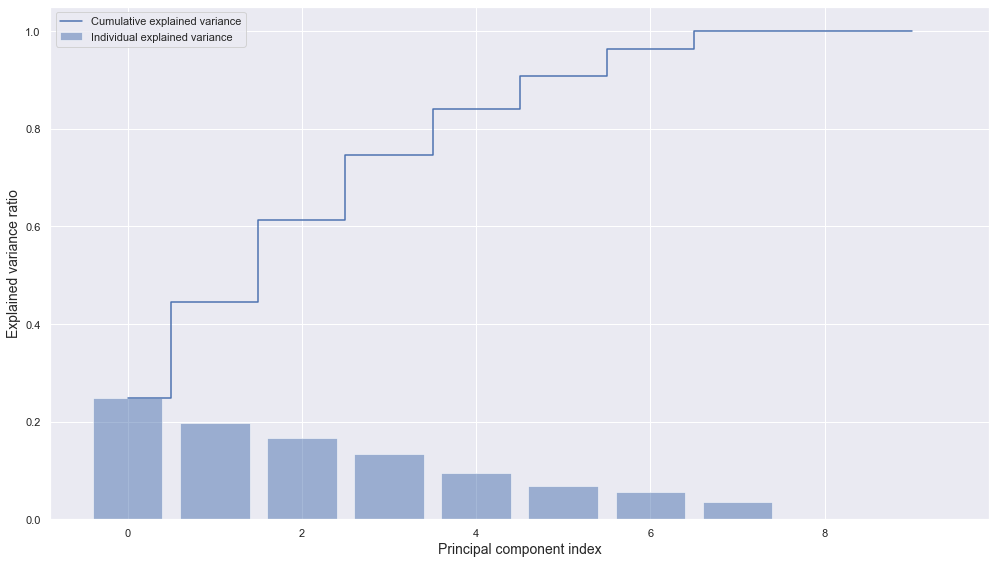
• 4 PC variables can explain almost 80% of total variance.

X_pca[:, :2].shape

(891, 2)

X_pca_scatter = pd.concat([pd.DataFrame(X_pca[:, :2], columns = ["PC1", "PC2"]), pd.DataFrame(titanic_original.is_survived, columns = ["is_survived"])], axis = 1)
X_pca_scatter.head()

	PC1	PC2	is_survived
0	-1.549197	-0.628395	0
1	3.156084	1.732145	1
2	0.455716	-1.295524	1
3	1.562384	-0.519725	1
4	-1.695137	0.025692	0

plt.figure(figsize = (14, 8))
sns.scatterplot(data = X_pca_scatter, x = "PC1", y = "PC2", hue = "is_survived")
plt.xlabel("PC1", fontsize = 14)
plt.ylabel("PC2", fontsize = 14)
plt.show()

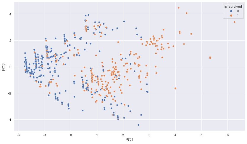
• It can be seen that we can classify well with PC1, PC2 values.
  -> Let’s do classification with PC1, PC2 variables.

X_pca[:, :2].shape

(891, 2)

X_pca_prep = X_pca[:, :2]

X_train, X_test, y_train, y_test = train_test_split(X_pca_prep, y, test_size = 0.1, random_state = 42)

names = ["Nearest Neighbors", 
         "Linear SVM", 
         "RBF SVM", 
         "Gaussian Process",
         "Decision Tree", 
         "Random Forest", 
         "Neural Net", 
         "AdaBoost",
         "Naive Bayes"
        ]

classifiers = [
    KNeighborsClassifier(3),
    SVC(kernel="linear", C=0.025),
    SVC(gamma=2, C=1),
    GaussianProcessClassifier(1.0 * RBF(1.0)),
    DecisionTreeClassifier(max_depth=5),
    RandomForestClassifier(max_depth=5, n_estimators=10, max_features=1),
    MLPClassifier(alpha=1, max_iter=1000),
    AdaBoostClassifier(),
    GaussianNB(),
    ]

for name, clf in zip(names, classifiers):
    try:
        clf.fit(X_train, y_train)
    except:
        clf.fit(X_train.toarray(), y_train)
    
    try:
        y_pred = clf.predict(X_test)
    except: 
        y_pred = clf.predict(X_test.toarray())
    
    # evaluate predictions
    try:
        accuracy = clf.score(X_test, y_test)
    except:
        accuracy = clf.score(X_test.toarray(), y_test)
    
    result_accuracy.loc[result_accuracy.model_name == name, "pca_accuracy"] = round(accuracy * 100, 3)
    #print(f"{name} Accuracy: {round(accuracy * 100, 3)}")

result_accuracy

	model_name	base_accuracy	pca_accuracy
0	Nearest Neighbors	83.333	81.111
1	Linear SVM	81.111	80.000
2	RBF SVM	81.111	82.222
3	Gaussian Process	83.333	80.000
4	Decision Tree	76.667	82.222
5	Random Forest	82.222	81.111
6	Neural Net	76.667	78.889
7	AdaBoost	82.222	78.889
8	Naive Bayes	78.889	81.111

• By using only PC1 and PC2 variables, we can obtain as high accuracy as baseline models.
• In some models like RBF SVM, Decision Tree, Neural Net, Naive Bayes, PCA variables got higher accuracy than baseline models.

TSNE

Let’s do TSNE and use variabels from TSNE instead of original columns.

X_original_prep.shape

(891, 10)

fig, ax = plt.subplots(3, 2, figsize = (15, 20))
for i, perplexity in enumerate([1, 5, 10, 15, 25, 35]):
    tsne = TSNE(n_components = 2, random_state = 42, perplexity = perplexity)
    X_2d = tsne.fit_transform(X_original_prep)
    tsne_labelled = pd.concat([pd.DataFrame(X_2d, columns = ["d1", "d2"]), titanic_original[["is_survived"]].astype(str)], axis = 1)
    
    sns.scatterplot(data = tsne_labelled, x = "d1", y = "d2", hue = "is_survived", ax = ax[i // 2, i % 2])
    ax[i // 2, i % 2].set_title(f"Perplexity = {perplexity}", fontsize = 14)

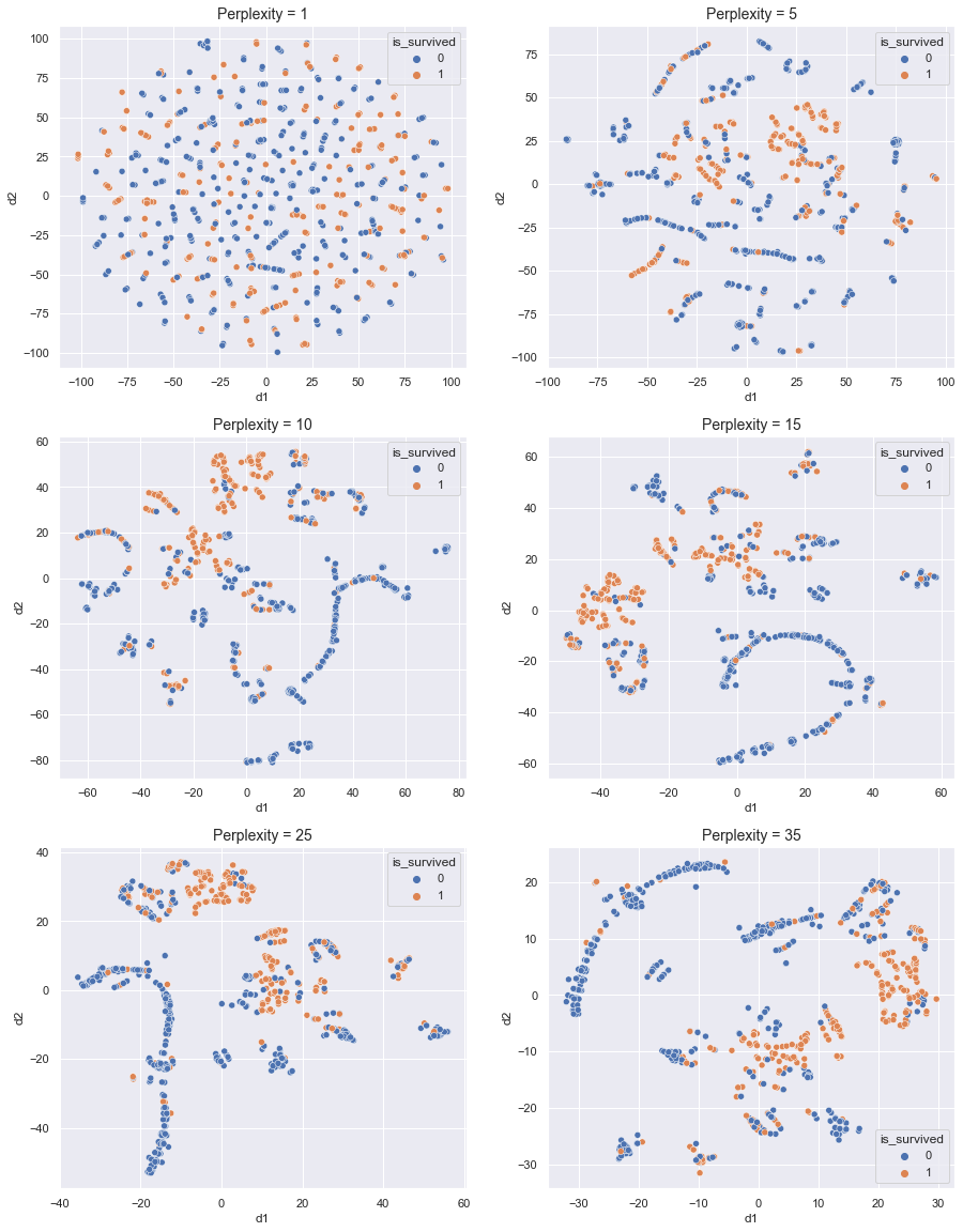
• From perplexity 15, we can figure out some distinct clusters. And some clusters have a higher rate of survival.
  -> Let’s use higher perplexities.

fig, ax = plt.subplots(3, 2, figsize = (15, 20))
for i, perplexity in enumerate([15, 25, 30, 35, 40, 45]):
    tsne = TSNE(n_components = 2, random_state = 42, perplexity = perplexity)
    X_2d = tsne.fit_transform(X_original_prep)
    tsne_labelled = pd.concat([pd.DataFrame(X_2d, columns = ["d1", "d2"]), titanic_original[["is_survived"]].astype(str)], axis = 1)
    
    sns.scatterplot(data = tsne_labelled, x = "d1", y = "d2", hue = "is_survived", ax = ax[i // 2, i % 2])
    ax[i // 2, i % 2].set_title(f"Perplexity = {perplexity}", fontsize = 14)

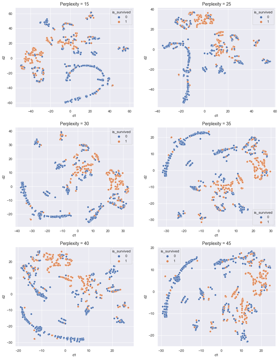
• From 15, the results are almost similar to each other.
• When perplexity is 25, the distinction between clusters was clear.
  -> Let’s use perplexity = 25

tsne = TSNE(n_components = 2, random_state = 42, perplexity = 25)
X_tsne_prep = tsne.fit_transform(X_original_prep)

X_train, X_test, y_train, y_test = train_test_split(X_tsne_prep, y, test_size = 0.1, random_state = 42)

names = ["Nearest Neighbors", 
         "Linear SVM", 
         "RBF SVM", 
         "Gaussian Process",
         "Decision Tree", 
         "Random Forest", 
         "Neural Net", 
         "AdaBoost",
         "Naive Bayes"
        ]

classifiers = [
    KNeighborsClassifier(3),
    SVC(kernel="linear", C=0.025),
    SVC(gamma=2, C=1),
    GaussianProcessClassifier(1.0 * RBF(1.0)),
    DecisionTreeClassifier(max_depth=5),
    RandomForestClassifier(max_depth=5, n_estimators=10, max_features=1),
    MLPClassifier(alpha=1, max_iter=1000),
    AdaBoostClassifier(),
    GaussianNB(),
    ]

for name, clf in zip(names, classifiers):
    try:
        clf.fit(X_train, y_train)
    except:
        clf.fit(X_train.toarray(), y_train)
    
    try:
        y_pred = clf.predict(X_test)
    except: 
        y_pred = clf.predict(X_test.toarray())
    
    # evaluate predictions
    try:
        accuracy = clf.score(X_test, y_test)
    except:
        accuracy = clf.score(X_test.toarray(), y_test)
    
    result_accuracy.loc[result_accuracy.model_name == name, "tsne_accuracy"] = round(accuracy * 100, 3)
    #print(f"{name} Accuracy: {round(accuracy * 100, 3)}")

result_accuracy

	model_name	base_accuracy	pca_accuracy	tsne_accuracy
0	Nearest Neighbors	83.333	81.111	81.111
1	Linear SVM	81.111	80.000	73.333
2	RBF SVM	81.111	82.222	81.111
3	Gaussian Process	83.333	80.000	82.222
4	Decision Tree	76.667	82.222	83.333
5	Random Forest	82.222	81.111	83.333
6	Neural Net	76.667	78.889	76.667
7	AdaBoost	82.222	78.889	76.667
8	Naive Bayes	78.889	81.111	73.333

• By using only 2 variables from tsne, we can obtain as high accuracy as baseline models.
• In Decision Tree and Random Forest, tsne variables got the highest accuracy than baseline or PCA models.

3.3. EDA variables

Now, let’s use variables from EDA and compare the accuracy with accuracies from methods used before.

titanic.head()

	is_survived	p_class	name	sex	age	num_sb_sp	num_pr_ch	ticket_number	ticket_fare	cabin_number	embark_port	ticket_number_alphabet	ticket_number_number	num_cmp	ticket_fare_category	cabin_alphabet	name_title	age_category	ticket_fare_category_order	age_category_order
0	0	3	Braund, Mr. Owen Harris	male	22.0	1	0	A/5 21171	7.2500	NaN	S	A/5	21171	1	(4.010999999999999, 8.676]	n	Mr	(16.336, 24.294]	1.0	3.0
1	1	1	Cumings, Mrs. John Bradley (Florence Briggs Th...	female	38.0	1	0	PC 17599	71.2833	C85	C	PC	17599	1	(26.25, 512.329]	C	Mrs	(32.252, 40.21]	3.0	5.0
2	1	3	Heikkinen, Miss. Laina	female	26.0	0	0	STON/O2. 3101282	7.9250	NaN	S	STON/O2.	3101282	0	(4.010999999999999, 8.676]	n	Miss	(24.294, 32.252]	1.0	4.0
3	1	1	Futrelle, Mrs. Jacques Heath (Lily May Peel)	female	35.0	1	0	113803	53.1000	C123	S	non	113803	1	(26.25, 512.329]	C	Mrs	(32.252, 40.21]	3.0	5.0
4	0	3	Allen, Mr. William Henry	male	35.0	0	0	373450	8.0500	NaN	S	non	373450	0	(4.010999999999999, 8.676]	n	Mr	(32.252, 40.21]	1.0	5.0

titanic.info()

<class 'pandas.core.frame.DataFrame'>
Int64Index: 891 entries, 0 to 890
Data columns (total 20 columns):
 #   Column                      Non-Null Count  Dtype   
---  ------                      --------------  -----   
 0   is_survived                 891 non-null    int64   
 1   p_class                     891 non-null    int64   
 2   name                        891 non-null    object  
 3   sex                         891 non-null    object  
 4   age                         891 non-null    float64 
 5   num_sb_sp                   891 non-null    int64   
 6   num_pr_ch                   891 non-null    int64   
 7   ticket_number               891 non-null    object  
 8   ticket_fare                 891 non-null    float64 
 9   cabin_number                204 non-null    object  
 10  embark_port                 891 non-null    object  
 11  ticket_number_alphabet      891 non-null    object  
 12  ticket_number_number        891 non-null    object  
 13  num_cmp                     891 non-null    int64   
 14  ticket_fare_category        891 non-null    category
 15  cabin_alphabet              891 non-null    object  
 16  name_title                  891 non-null    object  
 17  age_category                714 non-null    category
 18  ticket_fare_category_order  891 non-null    float64 
 19  age_category_order          891 non-null    float64 
dtypes: category(2), float64(4), int64(5), object(9)
memory usage: 166.9+ KB

X = titanic.drop(["is_survived", "name", "ticket_number", "cabin_number", "ticket_number_alphabet", \
                  "ticket_number_number", "cabin_alphabet", "ticket_fare_category", "age_category"], axis = 1)
y = titanic["is_survived"]

X

	p_class	sex	age	num_sb_sp	num_pr_ch	ticket_fare	embark_port	num_cmp	name_title	ticket_fare_category_order	age_category_order
0	3	male	22.000000	1	0	7.2500	S	1	Mr	1.0	3.0
1	1	female	38.000000	1	0	71.2833	C	1	Mrs	3.0	5.0
2	3	female	26.000000	0	0	7.9250	S	0	Miss	1.0	4.0
3	1	female	35.000000	1	0	53.1000	S	1	Mrs	3.0	5.0
4	3	male	35.000000	0	0	8.0500	S	0	Mr	1.0	5.0
...	...	...	...	...	...	...	...	...	...	...	...
886	2	male	27.000000	0	0	13.0000	S	0	uncommon	2.0	4.0
887	1	female	19.000000	0	0	30.0000	S	0	Miss	3.0	3.0
888	3	female	15.685263	1	2	23.4500	S	3	Miss	2.0	2.0
889	1	male	26.000000	0	0	30.0000	C	0	Mr	3.0	4.0
890	3	male	32.000000	0	0	7.7500	Q	0	Mr	1.0	4.0

891 rows × 11 columns

num_features = ["p_class", "age", "num_sb_sp", "num_pr_ch", "ticket_fare", "num_cmp", "ticket_fare_category_order", "age_category_order"]
nonnum_features = ["sex", "embark_port", "name_title"]

full_pipeline = ColumnTransformer([
    ("num", StandardScaler(), num_features),
    ("nonnum", OneHotEncoder(), nonnum_features),
])

X_eda_prep = full_pipeline.fit_transform(X)

X_train, X_test, y_train, y_test = train_test_split(X_eda_prep, y, test_size = 0.1, random_state = 42)

names = ["Nearest Neighbors", 
         "Linear SVM", 
         "RBF SVM", 
         "Gaussian Process",
         "Decision Tree", 
         "Random Forest", 
         "Neural Net", 
         "AdaBoost",
         "Naive Bayes"
        ]

classifiers = [
    KNeighborsClassifier(3),
    SVC(kernel="linear", C=0.025),
    SVC(gamma=2, C=1),
    GaussianProcessClassifier(1.0 * RBF(1.0)),
    DecisionTreeClassifier(max_depth=5),
    RandomForestClassifier(max_depth=5, n_estimators=10, max_features=1),
    MLPClassifier(alpha=1, max_iter=1000),
    AdaBoostClassifier(),
    GaussianNB(),
    ]

for name, clf in zip(names, classifiers):
    try:
        clf.fit(X_train, y_train)
    except:
        clf.fit(X_train.toarray(), y_train)
    
    try:
        y_pred = clf.predict(X_test)
    except: 
        y_pred = clf.predict(X_test.toarray())
    
    # evaluate predictions
    try:
        accuracy = clf.score(X_test, y_test)
    except:
        accuracy = clf.score(X_test.toarray(), y_test)
    
    result_accuracy.loc[result_accuracy.model_name == name, "eda_variables"] = round(accuracy * 100, 3)
    #print(f"{name} Accuracy: {round(accuracy * 100, 3)}")

result_accuracy

	model_name	base_accuracy	pca_accuracy	tsne_accuracy	eda_variables
0	Nearest Neighbors	83.333	81.111	81.111	84.444
1	Linear SVM	81.111	80.000	73.333	82.222
2	RBF SVM	81.111	82.222	81.111	80.000
3	Gaussian Process	83.333	80.000	82.222	84.444
4	Decision Tree	76.667	82.222	83.333	83.333
5	Random Forest	82.222	81.111	83.333	80.000
6	Neural Net	76.667	78.889	76.667	80.000
7	AdaBoost	82.222	78.889	76.667	82.222
8	Naive Bayes	78.889	81.111	73.333	78.889

• In Nearest Neighbors, Linear SVM, Gaussian Process, AdaBoost, eda variables got the highest accuracy than other methods.
  -> Let’s tune Nearest Neighbors, Linear SVM, Gaussian Process, Deicision Tree, and Random Forest and ensemble these models.

3.4. Hyperparameter Tuning

Let’s tune the hyperparameters for each of 5 models that I will use: Nearest Neighbors, Linear SVM, Gaussian Process, Deicision Tree, and Random Forest.

Nearest Neighbors

param_grid = {
    'leaf_size': [1, 3, 5, 7, 9],
    'n_neighbors': [1, 3, 5, 7, 9],
    'p' : [1,2]
}

model = KNeighborsClassifier()

eda_knn_grid = GridSearchCV(model, param_grid, cv = 5, n_jobs = -1)
eda_knn_grid.fit(X_eda_prep, y)

print(eda_knn_grid.best_estimator_)
print(eda_knn_grid.best_score_)

KNeighborsClassifier(leaf_size=1, n_neighbors=7)
0.8237838177138912

• Best parameters: leaf_size = 1, n_neighbors = 7
• Best score: about 82%

Linear SVM

param_grid = {
    'C': [0.1, 1, 10, 100],
    'gamma': [1, 0.1, 0.01],
}

model = SVC(kernel = "linear")

eda_svm_grid = GridSearchCV(model, param_grid, cv = 5, n_jobs = -1)
eda_svm_grid.fit(X_eda_prep, y)

print(eda_svm_grid.best_estimator_)
print(eda_svm_grid.best_score_)

SVC(C=0.1, gamma=1, kernel='linear')
0.8248948590797817

• Best parameters: c = 0.1, gamma = 1
• Best score: about 82%

Gaussian Process

param_grid = {
    "kernel": [1 * RBF(), 1 * DotProduct(), 1 * Matern(),  1 * RationalQuadratic(), 1 * WhiteKernel()]
}

model = GaussianProcessClassifier()

eda_gaussian_grid = GridSearchCV(model, param_grid, cv = 5, n_jobs = -1)
eda_gaussian_grid.fit(X_eda_prep, y)

print(eda_gaussian_grid.best_estimator_)
print(eda_gaussian_grid.best_score_)

/opt/anaconda3/lib/python3.9/site-packages/sklearn/gaussian_process/kernels.py:411: ConvergenceWarning: The optimal value found for dimension 0 of parameter k2__alpha is close to the specified upper bound 100000.0. Increasing the bound and calling fit again may find a better value.
  warnings.warn("The optimal value found for "
/opt/anaconda3/lib/python3.9/site-packages/sklearn/gaussian_process/kernels.py:411: ConvergenceWarning: The optimal value found for dimension 0 of parameter k2__alpha is close to the specified upper bound 100000.0. Increasing the bound and calling fit again may find a better value.
  warnings.warn("The optimal value found for "


GaussianProcessClassifier(kernel=1**2 * RBF(length_scale=1))
0.8271608813006089

• Best parameters: kernel = 1 ** 2 * RBF(length_scale = 1)
• Best score: about 83%

Decision tree

param_grid = {
    "splitter":["best","random"],
    "max_depth" : [1,3,5,7,9],
    "min_samples_leaf":[1,2,3],
    "min_weight_fraction_leaf":[0.1,0.2,0.3,0.4],
    "max_features":["auto","log2","sqrt",None],
    "max_leaf_nodes":[None, 20, 40, 60]
}

model = DecisionTreeClassifier()

eda_decision_tree_grid = GridSearchCV(model, param_grid, cv = 5, n_jobs = -1)
eda_decision_tree_grid.fit(X_eda_prep, y)

print(eda_decision_tree_grid.best_estimator_)
print(eda_decision_tree_grid.best_score_)

DecisionTreeClassifier(max_depth=9, max_features='auto', max_leaf_nodes=40,
                       min_samples_leaf=2, min_weight_fraction_leaf=0.2)
0.7968740192078337

• Best parameters: max_depth = 7, max_features = “sqrt”, max_leaf_nodes = 60, min_samples_leaf = 3, min_weight_fraction_leaf = 0.1
• Best score: about 80%

Random forest

param_grid = {
    'bootstrap': [True, False],
    'max_depth': [10, 30, 50],
    'max_features': ['auto', 'sqrt'],
    'min_samples_leaf': [1, 2, 4],
    'min_samples_split': [2, 5, 10],
    'n_estimators': [5, 10, 15, 20]
}

model = RandomForestClassifier()

eda_random_forest_grid = GridSearchCV(model, param_grid, cv = 5, n_jobs = -1)
eda_random_forest_grid.fit(X_eda_prep, y)

print(eda_random_forest_grid.best_estimator_)
print(eda_random_forest_grid.best_score_)

RandomForestClassifier(max_depth=30, max_features='sqrt', min_samples_leaf=2,
                       min_samples_split=5, n_estimators=20)
0.8439834285355596

• Best parameters: bootstrap = False, max_depth = 10, miin_samples_leaf = 4, min_samples_split = 10, n_estimators = 15
• Best score: about 85%

3.5. Ensemble Models

Now, let’s tune classfiers and ensemble these models.

Nearest Neighbors, Linear SVM, Gaussian Process

X = titanic.drop(["is_survived", "name", "ticket_number", "cabin_number", "ticket_number_alphabet", \
                  "ticket_number_number", "cabin_alphabet", "ticket_fare_category", "age_category"], axis = 1)
y = titanic["is_survived"]

num_features = ["p_class", "age", "num_sb_sp", "num_pr_ch", "ticket_fare", "num_cmp", "ticket_fare_category_order", "age_category_order"]
nonnum_features = ["sex", "embark_port", "name_title"]

full_pipeline = ColumnTransformer([
    ("num", StandardScaler(), num_features),
    ("nonnum", OneHotEncoder(), nonnum_features),
])

X_eda_prep = full_pipeline.fit_transform(X)

X_train, X_test, y_train, y_test = train_test_split(X_eda_prep, y, test_size = 0.1, random_state = 42)

clf_knn = KNeighborsClassifier(leaf_size = eda_knn_grid.best_params_["leaf_size"], n_neighbors = eda_knn_grid.best_params_["n_neighbors"])

clf_svc = SVC(kernel = "linear", C = eda_svm_grid.best_params_["C"], gamma = eda_svm_grid.best_params_["gamma"])

clf_gaussian_process = GaussianProcessClassifier(kernel = eda_gaussian_grid.best_params_["kernel"])


clf_decision_tree = DecisionTreeClassifier(
    max_depth = eda_decision_tree_grid.best_params_["max_depth"],
    max_features = eda_decision_tree_grid.best_params_["max_features"],
    max_leaf_nodes = eda_decision_tree_grid.best_params_["max_leaf_nodes"],
    min_samples_leaf = eda_decision_tree_grid.best_params_["min_samples_leaf"],
    min_weight_fraction_leaf = eda_decision_tree_grid.best_params_["min_weight_fraction_leaf"],
    splitter = eda_decision_tree_grid.best_params_["splitter"],
)

clf_random_forest = RandomForestClassifier(
    bootstrap = eda_random_forest_grid.best_params_["bootstrap"],
    max_depth = eda_random_forest_grid.best_params_["max_depth"],
    max_features = eda_random_forest_grid.best_params_["max_features"],
    min_samples_leaf = eda_random_forest_grid.best_params_["min_samples_leaf"],
    min_samples_split = eda_random_forest_grid.best_params_["min_samples_split"],
    n_estimators = eda_random_forest_grid.best_params_["n_estimators"],
)

clf_ensemble = VotingClassifier(
    estimators = [("knn", clf_knn), ("svc", clf_svc), ("gp", clf_gaussian_process),
                  ("dt", clf_decision_tree), ("rf", clf_random_forest)], 
    voting = "hard"
)

clf_ensemble = clf_ensemble.fit(X_train, y_train)
y_pred = clf_ensemble.predict(X_test)
accuracy = clf_ensemble.score(X_test, y_test)

round(accuracy * 100, 3)

82.222

• Get about 82% accuracy from the ensemble model.

4. Prepare submission

X.head()

	p_class	sex	age	num_sb_sp	num_pr_ch	ticket_fare	embark_port	num_cmp	name_title	ticket_fare_category_order	age_category_order
0	3	male	22.0	1	0	7.2500	S	1	Mr	1.0	3.0
1	1	female	38.0	1	0	71.2833	C	1	Mrs	3.0	5.0
2	3	female	26.0	0	0	7.9250	S	0	Miss	1.0	4.0
3	1	female	35.0	1	0	53.1000	S	1	Mrs	3.0	5.0
4	3	male	35.0	0	0	8.0500	S	0	Mr	1.0	5.0

test = test[X.columns]
test.head()

	p_class	sex	age	num_sb_sp	num_pr_ch	ticket_fare	embark_port	num_cmp	name_title	ticket_fare_category_order	age_category_order
0	3	male	34.5	0	0	7.8292	Q	0	Mr	1.0	5.0
1	3	female	47.0	1	0	7.0000	S	1	Mrs	1.0	6.0
2	2	male	62.0	0	0	9.6875	Q	0	Mr	2.0	8.0
3	3	male	27.0	0	0	8.6625	S	0	Mr	1.0	4.0
4	3	female	22.0	1	1	12.2875	S	2	Mrs	2.0	3.0

test.info()

<class 'pandas.core.frame.DataFrame'>
Int64Index: 418 entries, 0 to 417
Data columns (total 11 columns):
 #   Column                      Non-Null Count  Dtype  
---  ------                      --------------  -----  
 0   p_class                     418 non-null    int64  
 1   sex                         418 non-null    object 
 2   age                         418 non-null    float64
 3   num_sb_sp                   418 non-null    int64  
 4   num_pr_ch                   418 non-null    int64  
 5   ticket_fare                 418 non-null    float64
 6   embark_port                 418 non-null    object 
 7   num_cmp                     418 non-null    int64  
 8   name_title                  418 non-null    object 
 9   ticket_fare_category_order  418 non-null    float64
 10  age_category_order          418 non-null    float64
dtypes: float64(4), int64(4), object(3)
memory usage: 39.2+ KB

X_submission_prep = full_pipeline.transform(test)

y_pred = clf_ensemble.predict(X_submission_prep)

submission = pd.DataFrame({
    "PassengerId": test_passenger_id,
    "Survived": y_pred
})

submission.head()

	PassengerId	Survived
0	892	0
1	893	1
2	894	0
3	895	0
4	896	1

#submission.to_csv('./data/titanic_submission.csv', index=False)