
HW1. KNN
Topics: EDA(Exploratory Data Analysis), KNN
import numpy as np
import pandas as pd

import matplotlib as mpl
import matplotlib.pyplot as plt
import seaborn as sns
import plotly.express as px
import missingno as msno

from sklearn.model_selection import train_test_split
from sklearn.preprocessing import StandardScaler
from sklearn.impute import SimpleImputer
from sklearn.experimental import enable_iterative_imputer
from sklearn.impute import IterativeImputer
from sklearn.neighbors import KNeighborsClassifier
from sklearn.metrics import confusion_matrix, ConfusionMatrixDisplay
Problem: KNN
Use the k-nearest neighbor classifier on the diabetes dataset. In particular, consider k = 1, 2, . . ., 30. Show both the training and test errors for each choice and report your findings. Hint: 1) Note the prediction/input variables are of different units and scales. Therefore, standardization is necessary before applying the KNN method. 2) Exploratory data analysis (EDA) is an important step to get familiar with the data and better understand it. Make sure you do it with every data analysis project.
1. EDA
Missing values
df_train = pd.read_csv("diabetes_train.csv")
df_test = pd.read_csv("diabetes_test.csv")
df_train.isna().sum()
Pregnancies                 0
Glucose                     0
BloodPressure               0
SkinThickness               0
Insulin                     0
BMI                         0
DiabetesPedigreeFunction    0
Age                         0
Outcome                     0
dtype: int64
df_test.isna().sum()
Pregnancies                 0
Glucose                     0
BloodPressure               0
SkinThickness               0
Insulin                     0
BMI                         0
DiabetesPedigreeFunction    0
Age                         0
Outcome                     0
dtype: int64
It looks like there are no missing values in both train and test data.
df_train.describe()
| Pregnancies | Glucose | BloodPressure | SkinThickness | Insulin | BMI | DiabetesPedigreeFunction | Age | Outcome | |
|---|---|---|---|---|---|---|---|---|---|
| count | 428.000000 | 428.000000 | 428.000000 | 428.000000 | 428.000000 | 428.000000 | 428.000000 | 428.000000 | 428.000000 |
| mean | 4.053738 | 124.752336 | 69.672897 | 20.072430 | 84.067757 | 32.549065 | 0.502308 | 34.329439 | 0.478972 |
| std | 3.538270 | 32.822486 | 19.135913 | 16.555687 | 124.157706 | 7.669440 | 0.347304 | 11.926841 | 0.500142 |
| min | 0.000000 | 0.000000 | 0.000000 | 0.000000 | 0.000000 | 0.000000 | 0.078000 | 21.000000 | 0.000000 |
| 25% | 1.000000 | 103.000000 | 64.000000 | 0.000000 | 0.000000 | 27.875000 | 0.253750 | 25.000000 | 0.000000 |
| 50% | 3.000000 | 123.000000 | 72.000000 | 22.500000 | 0.000000 | 32.500000 | 0.402500 | 31.000000 | 0.000000 |
| 75% | 7.000000 | 145.000000 | 80.000000 | 32.000000 | 130.000000 | 36.800000 | 0.675000 | 41.250000 | 1.000000 |
| max | 17.000000 | 199.000000 | 114.000000 | 99.000000 | 846.000000 | 59.400000 | 2.420000 | 81.000000 | 1.000000 |
However, if we check the basic statistics of each variables, then some variables have 0 as minimum value, which is impossible for human. For instance, people cannot have 0 glucose concentration, insuline, blood pressure, skinthickness, and BMI. Let’s check these variables more.
target_columns = ["Glucose", "BloodPressure", "SkinThickness", "Insulin", "BMI"]

fig, axes = plt.subplots(1, len(target_columns), figsize = (15, 5))

for i, col in enumerate(target_columns):
    sns.boxplot(df_train.loc[:, col], ax = axes[i])
    axes[i].set_xlabel(col)
    axes[i].set_ylabel("Value")

plt.tight_layout()
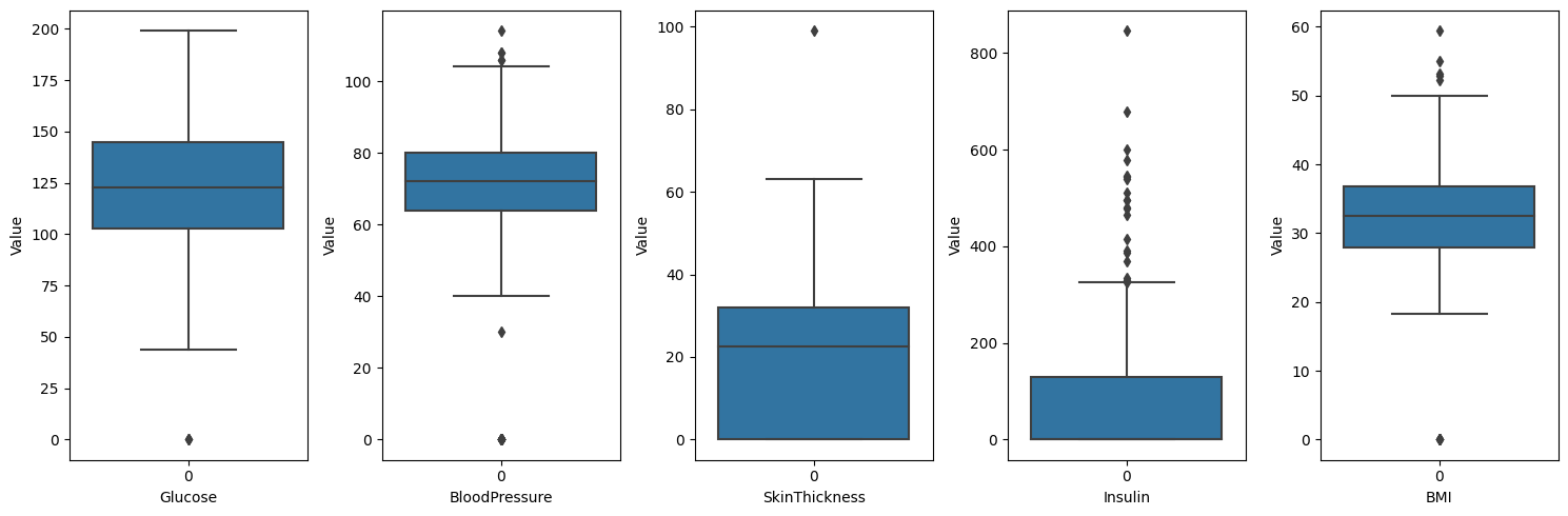
- Glucose, BloodPressure, BMI: when we check the distribution of data, it is abnormal to have value 0. So we can conclude that value 0 means missing value in these variables.
- SkinThickness, Insulin: Let’s take a closer look at these variables, as it is difficult to determine.
fig, axes = plt.subplots(1, 2, figsize = (15, 5))

sns.barplot(df_train.loc[df_train["SkinThickness"] < 15, "SkinThickness"].value_counts().sort_values().reset_index(),
            x = "index", y = "SkinThickness", ax = axes[0])
axes[0].set_xlabel("SkinThickness")
axes[0].set_ylabel("Count")

sns.barplot(df_train.loc[df_train["Insulin"] < 50, "Insulin"].value_counts().sort_values().reset_index(),
            x = "index", y = "Insulin", ax = axes[1])
axes[1].set_xlabel("Insulin")
axes[1].set_ylabel("Count")
Text(0, 0.5, 'Count')
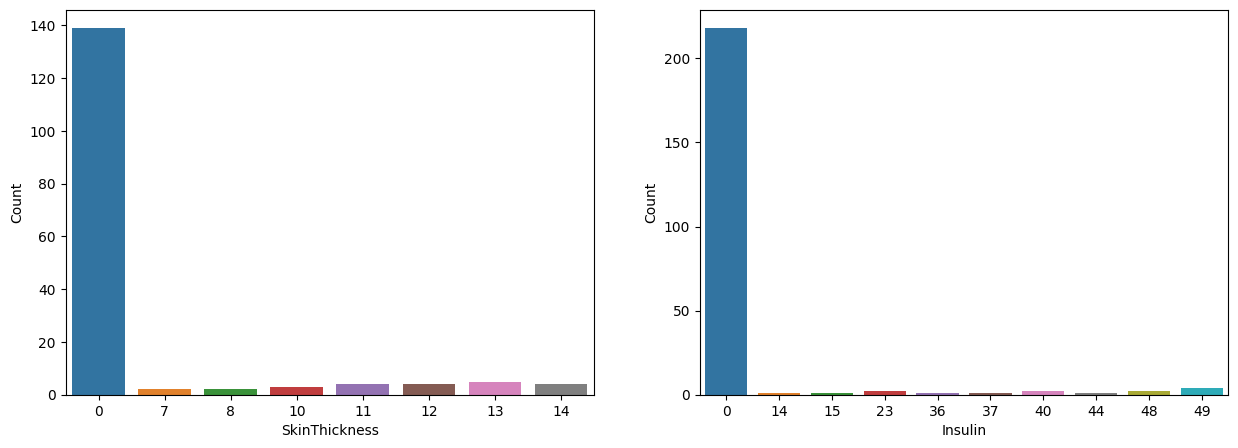
The above bar plots show the distribution of data with values near zero. When compared to non-zero data, it can be seen that having 0 is abnormal in both variables. So we can conclude that value 0 means missing value in these variables.
Let’s replace 0 to the missing value in Blucose, BloodPressure, SkinThickness, Insuline, BMI variables
target_columns = ["Glucose", "BloodPressure", "SkinThickness", "Insulin", "BMI"]

for col in target_columns:
    df_train.loc[df_train[col] == 0, col] = np.nan
    df_test.loc[df_test[col] == 0, col] = np.nan
print("The number of nan values in training data:")
for col in target_columns:
    print(f"- {col}: ", np.sum(df_train[col].isna()))

print(" ")
print("The number of nan values in test data:")
for col in target_columns:
    print(f"- {col}: ", np.sum(df_test[col].isna()))
The number of nan values in training data:
- Glucose:  3
- BloodPressure:  19
- SkinThickness:  139
- Insulin:  218
- BMI:  6

The number of nan values in test data:
- Glucose:  1
- BloodPressure:  9
- SkinThickness:  32
- Insulin:  51
- BMI:  1
fig, axes = plt.subplots(1, 2, figsize = (15, 8))
msno.bar(df_train, ax = axes[0])
msno.bar(df_test, ax = axes[1])
axes[0].set_title("Train data", fontsize = 25)
axes[1].set_title("Test data", fontsize = 25)
plt.tight_layout()
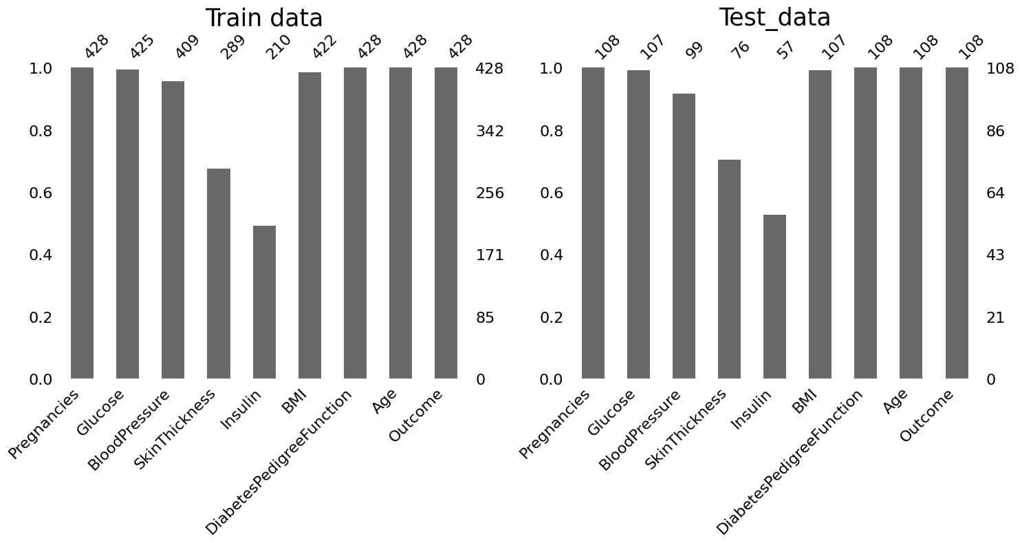
Above print results and bar plots show how many missing values there are for each variables in train and test data.
- Glucose, BMI, BloodPressure: have very few missing values. Less than 5% for train data and less than 10% for test data.
- SkinThickness, Insuline: have very many missing values. Over 30% for both train and test data.
fig, axes = plt.subplots(1, 2, figsize = (20, 8))
msno.matrix(df_train, figsize = (12, 4), ax = axes[0])
msno.matrix(df_test, figsize = (12, 4), ax = axes[1])
axes[0].set_title("Train data", fontsize = 25)
axes[1].set_title("Test data", fontsize = 25)
plt.tight_layout()
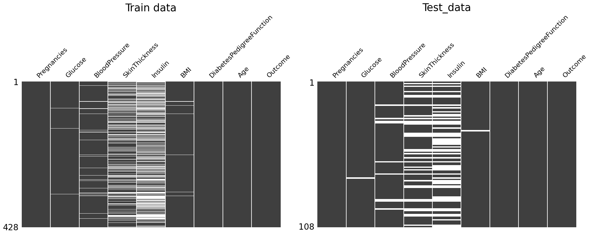
We can check the pattern of missingness in the dataset by above plots.
- Train data: If glucose is a missing value, it seems that all other 4 variables are also missing values.
- Test data: It seems that there is no pattern of missing values among 5 variables.
Distribution
sns.pairplot(df_train, diag_kind = "kde", hue = "Outcome")
<seaborn.axisgrid.PairGrid at 0x7fa924c7a278>
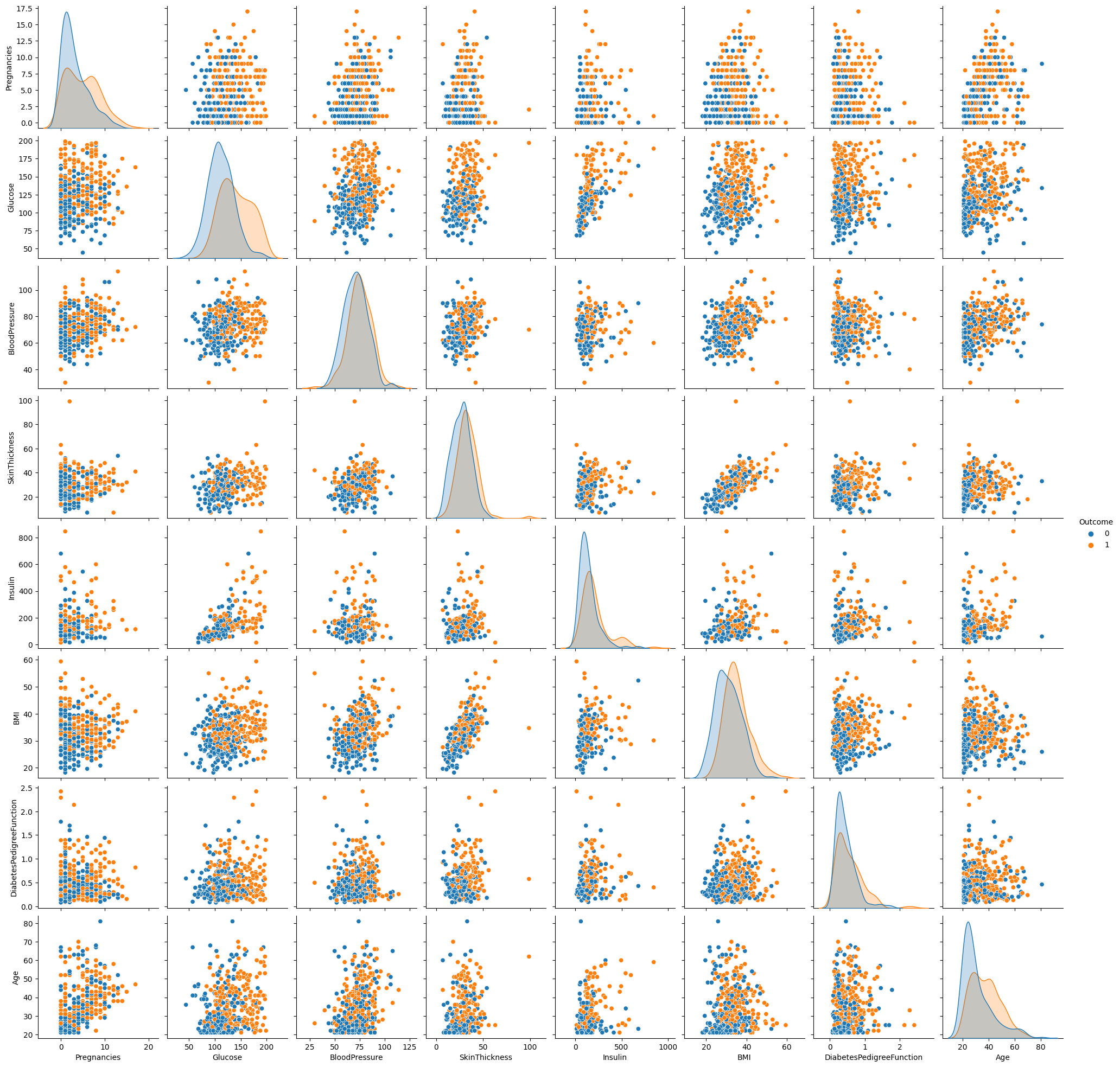
- When we check the kde plot of Glucose, it seems that the difference in distribution between Outcome = 1 and Outcome = 0 is larger than that of other variables.
- When we check all pairplots, in the pairplot of glucose and other variables, it is possible to better distinguish Outcome = 1 and Outcome = 0.
df_train_boxplot = df_train.copy()


px.box(df_train_boxplot.melt(id_vars=['Outcome'], var_name = "col" ), x = "Outcome", y='value',
       color = 'Outcome',facet_col='col').update_yaxes(matches=None)
- As seen in the kde plot of pairplot, there seems to be a significant difference between the distribution of Outcome = 0 and Outcome = 1 for Glucose.
- In the case of SkinThickness and Insulin, which have many missing values, there is no clear difference in the distribution of Outcome = 0 and Outcome = 1.
Correlation
corr = df_train.corr()
mask = np.triu(np.ones_like(corr, dtype=bool))

sns.heatmap(corr, mask = mask, annot = True, cmap = "BrBG", vmin = -1, vmax = 1, linewidths = 0.5, cbar_kws = {"shrink" : 0.5})
<AxesSubplot:>
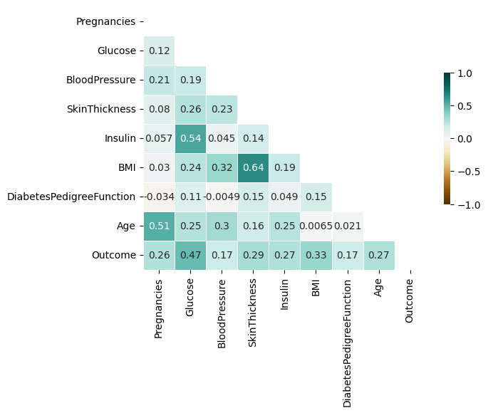
- Most of the variables show positive correlations.
- There are quite high correlations between Insulin & Glucose / BMI & SkinThickness / Age & Pregnancies.
- Outcome has highest correlation of 0.47 with Glucose, which is the ssame result as above.
- SkinThickness and Insuline have not that high correlation with Outcome.
We have check that Since SkinThickness and Insuline have many missing values and contain few information about Outcome. Also Skinthickness has high correlation with BMI and Insulin has high correlation with Glucose. I think that the information of Insulin and SkinThickness can be sufficiently covered by Glucose and BMI alone respectively. So let’s proceed with the analysis without the Skinthickness and Insulin variables.
df_train = df_train.drop(["SkinThickness", "Insulin"], axis = 1)
df_test = df_test.drop(["SkinThickness", "Insulin"], axis = 1)
2. KNN without SkinThickness & Insulin
def my_knn(df_train, df_test, k_range, method, verbose = False, plot = False):
    # (0) Make base dataset
    if method == "dropna":
        df_train = df_train.dropna()
        df_test = df_test.dropna()

    X_train = df_train.drop(['Outcome'], axis=1)
    y_train = df_train['Outcome']
    X_test = df_test.drop(['Outcome'], axis=1)
    y_test = df_test['Outcome']

    columns = X_train.columns

    if method == "mean":
        imp = SimpleImputer(missing_values = np.nan, strategy = 'mean')

    elif method == "median":
        imp = SimpleImputer(missing_values=np.nan, strategy = 'median')

    elif method == "mice":
        imp = IterativeImputer(max_iter=10, random_state=42)

    if method != "dropna":
        X_train = imp.fit_transform(X_train)
        X_test = imp.fit_transform(X_test)

    if verbose == True:
        print("Method: ", method)
        print("Datasets are ready:")
        print("-- X_train: ", X_train.shape)
        print("-- y_train: ", y_train.shape)
        print("-- X_test: ", X_test.shape)
        print("-- y_test: ", y_test.shape)
        print("")

    # (1) Standardization
    scaler = StandardScaler()
    scaler.fit(X_train)

    X_train = scaler.transform(X_train)
    X_test = scaler.transform(X_test)

    if verbose == True:
        print("Datas are standardized: ")
        print("-- X_train: ")
        print(pd.DataFrame(X_train, columns = columns).describe())
        print("-- X_test: ")
        print(pd.DataFrame(X_test, columns = columns).describe())
        print("")

    # (2) KNN with varing K
    train_error = []
    test_error = []

    for k in k_range:
        # setup a knn classifier with k neighbors
        knn = KNeighborsClassifier(n_neighbors=k)

        # fit the model
        knn.fit(X_train, y_train)

        # train error rate
        pred_train = knn.predict(X_train)
        train_error.append(np.mean(pred_train != y_train))

        # test error rate
        pred_test = knn.predict(X_test)
        test_error.append(np.mean(pred_test != y_test))

    # (3) Plotting error rate curves
    if plot == True:
        plt.plot(1/k_range, train_error, label='Training Error')
        plt.plot(1/k_range, test_error, label='Test Error')
        plt.legend()
        plt.title('Training and test error rate for KNN')
        plt.xlabel('Number of neighbors (1 / k)')
        plt.ylabel('Error Rate')
        plt.show()

    return train_error, test_error
k_range = np.arange(1, 31)
fig, axes = plt.subplots(1, 4, figsize = (15, 5))

for i, method in enumerate(["dropna", "mean", "median", "mice"]):
    train_error, test_error = my_knn(df_train, df_test, k_range, method = method)

    axes[i].plot(1/k_range, train_error, label = "Training Error")
    axes[i].plot(1/k_range, test_error, label = "Test Error")

    axes[i].set_xlabel('Number of neighbors (1 / k)')
    axes[i].set_ylabel('Error Rate')

    if method == "dropna": axes[i].set_title("Drop missing values")
    elif method == "mean": axes[i].set_title("Impute missing values with mean")
    elif method == "median": axes[i].set_title("Impute missing values with median")
    elif method == "mice": axes[i].set_title("Impute missing values with MICE")

plt.tight_layout()
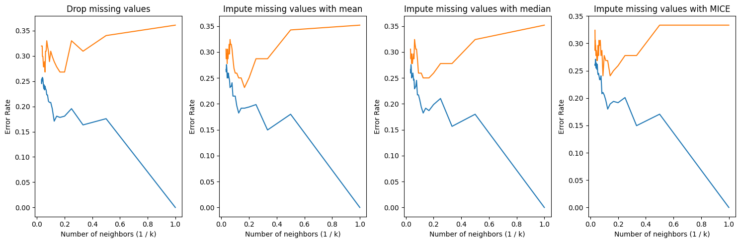
Above line graphs show train and test error results for each ways to handle missing values. We can obtain minimum error rate about 0.24 with 1/k about 0.2 when we impute missing values with mean.
3. KNN with Glucose & one other variable
As seen in the above EDA process, there was a some difference in the distribution of Outcomes = 0 and Outcomes = 1 in the case of Glucose.
fig, axes = plt.subplots(1, 5, figsize = (15, 5))

target_column = ["Pregnancies", "BloodPressure", "BMI", "DiabetesPedigreeFunction", "Age"]

for i, col in enumerate(target_column):
    sns.scatterplot(data = df_train[["Outcome", "Glucose", col]], x = "Glucose", y = col, hue = "Outcome", ax = axes[i])
plt.tight_layout()
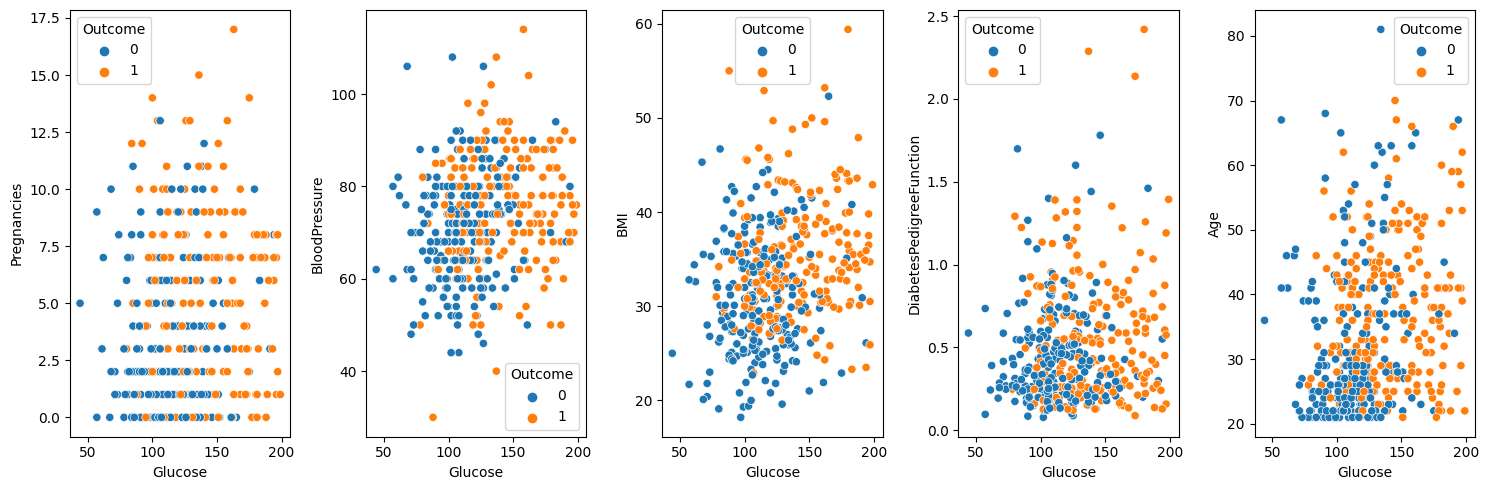
The plots above are scatter plots between Glucose and one other variable. If we look at the above plots, we can distinguish the Outcome = 0 group and Outcome = 1 group with our eyes to some extent. So, I want to try to apply KNN using only Glucose and one other variable and compare the results.
fig, axes = plt.subplots(4, 5, figsize = (15, 10))

for i, method in enumerate(["dropna", "mean", "median", "mice"]):
    if method == "dropna": y_label = "Drop NA"
    elif method == "mean": y_label = "Impute by mean"
    elif method == "median": y_label = "Impute by median"
    elif method == "mice": y_label = "Impute by MICE"

    axes[i, 0].set_ylabel(y_label, fontsize = 15)

    for j, col in enumerate(["Pregnancies", "BloodPressure", "BMI", "DiabetesPedigreeFunction", "Age"]):
        df_train_subset = df_train[["Outcome", "Glucose", col]]
        df_test_subset = df_test[["Outcome", "Glucose", col]]

        train_error, test_error = my_knn(df_train_subset, df_test_subset, k_range, method = method)

        axes[i, j].plot(1/k_range, train_error, label = "Training Error")
        axes[i, j].plot(1/k_range, test_error, label = "Test Error")

        if i == 0: axes[i, j].set_title(f'Glucose & {col}', fontsize = 15)

plt.tight_layout()
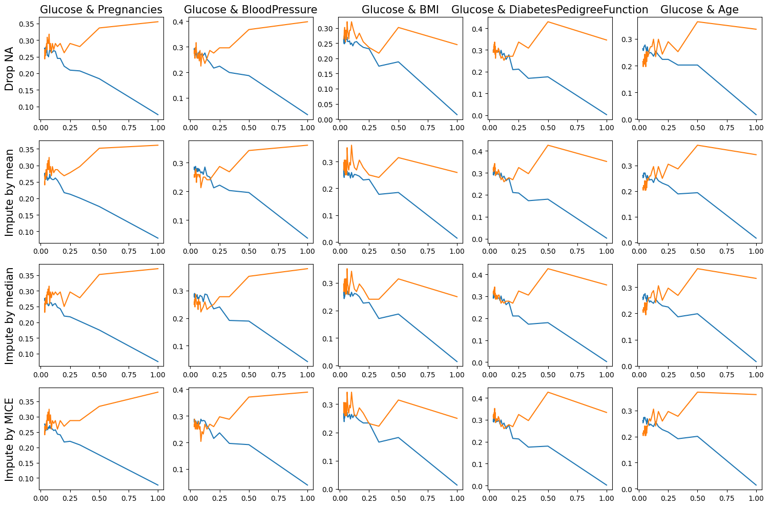
As we can see in the above training error and test error results, when using only two variables(Glucose & BloodPressure or Glucose & Age), a lower test error can be obtained than when using the rest of the above variables together.
4. Compare results
train_error_all, test_error_all = my_knn(df_train, df_test, k_range, method = "mean")

df_train_subset = df_train[["Outcome", "Glucose", "Age"]]
df_test_subset = df_test[["Outcome", "Glucose", "Age"]]
train_error_age, test_error_age = my_knn(df_train_subset, df_test_subset, k_range, method = "median")

df_train_subset = df_train[["Outcome", "Glucose", "BloodPressure"]]
df_test_subset = df_test[["Outcome", "Glucose", "BloodPressure"]]
train_error_bp, test_error_bp = my_knn(df_train_subset, df_test_subset, k_range, method = "mice")
plt.figure(figsize = (10, 5))
plt.plot(1/k_range, test_error_age, label = "Case 1: Glucose & Age / Median imputation")
plt.plot(1/k_range, test_error_bp, label = "Case 2: Glucose & BloodPressure / MICE imputation")
plt.plot(1/k_range, test_error_all, label = "Case 3: All variables / Mean imputation")
plt.vlines(1/k_range[np.argmin(test_error_age)], 0.15, 0.4, linestyles = "dashed", colors = "blue", alpha = 0.5)
plt.vlines(1/k_range[np.argmin(test_error_all)], 0.15, 0.4, linestyles = "dashed", colors = "green", alpha = 0.5)
plt.vlines(1/k_range[np.argmin(test_error_bp)], 0.15, 0.4, linestyles = "dashed", colors = "red", alpha = 0.5)

plt.xlabel('Number of neighbors (1 / k)')
plt.ylabel('Error Rate')
plt.title("Test Errors")

plt.legend(loc = 2)
<matplotlib.legend.Legend at 0x7fa90fe95cc0>
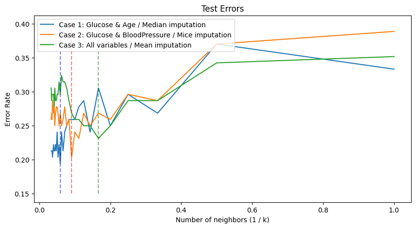
print("When we use")
print(f"- (case 1) Glocose & Age with median imputation, we can obtain minimum teset error = {round(np.min(test_error_age), 3)} when k = {k_range[np.argmin(test_error_age)]}")
print(f"- (case 2) Glocose & BloodPressure with MICE imputation, we can obtain minimum teset error = {round(np.min(test_error_bp), 3)} when k = {k_range[np.argmin(test_error_bp)]}")
print(f"- (case 3) all variables except SkinThickness and Insulin with mean imputation, we can obtain minimum teset error = {round(np.min(test_error_all), 3)} when k = {k_range[np.argmin(test_error_all)]}")
When we use
- (case 1) Glocose & Age with median imputation, we can obtain minimum teset error = 0.194 when k = 17
- (case 2) Glocose & BloodPressure with MICE imputation, we can obtain minimum teset error = 0.204 when k = 11
- (case 3) all variables except SkinThickness and Insulin with mean imputation, we can obtain minimum teset error = 0.231 when k = 6