
HW2. LDA, QDA, Naive Bayes
Topics: EDA(Exploratory Data Analysis), LDA(Linear Discriminant Analysis), QDA(Quadratic Discriminant Analysis), Naive Bayes
import pandas as pd
import numpy as np
import seaborn as sns
import matplotlib.pyplot as plt

from sklearn.discriminant_analysis import LinearDiscriminantAnalysis, QuadraticDiscriminantAnalysis
from sklearn.naive_bayes import GaussianNB
from sklearn.metrics import confusion_matrix
from sklearn.metrics import ConfusionMatrixDisplay
Problem: LDA, QDA, Naive Bayes
In this problem, you will develop models to predict the wine type based on the Wine data set.
(a) EDA
Explore the data graphically in order to investigate the association between Type and the other features. Which of the other features seem most likely to be useful in predicting Type? Scat- terplots and boxplots may be useful tools to answer this ques- tion. Describe your findings.
df_train = pd.read_csv("wine_train.csv")
df_test = pd.read_csv("wine_test.csv")
print(df_train.shape, df_test.shape)
(123, 14) (55, 14)
- train data: n = 123
- test data: n = 55
df_train.Type.value_counts()
2    49
1    41
3    33
Name: Type, dtype: int64
df_train.dtypes
Type                 int64
Alcohol            float64
Malic              float64
Ash                float64
Alcalinity         float64
Magnesium            int64
Phenols            float64
Flavanoids         float64
Nonflavanoids      float64
Proanthocyanins    float64
Color              float64
Hue                float64
Dilution           float64
Proline              int64
dtype: object
- independent variable:
- Type variable
- There are 3 types (1, 2, 3 types)
- The number of datas for each type are balanced. There are 41 type 1, 49 type 2, and 33 type 3.
- dependent variable: 13 variables
- All variables are numerical types.
Dependent variables Type is integer data type, so let’s change it to string.
df_train["Type"] = df_train["Type"].astype("string")
df_test["Type"] = df_test["Type"].astype("string")
df_train.isna().sum()
Type               0
Alcohol            0
Malic              0
Ash                0
Alcalinity         0
Magnesium          0
Phenols            0
Flavanoids         0
Nonflavanoids      0
Proanthocyanins    0
Color              0
Hue                0
Dilution           0
Proline            0
dtype: int64
df_test.isna().sum()
Type               0
Alcohol            0
Malic              0
Ash                0
Alcalinity         0
Magnesium          0
Phenols            0
Flavanoids         0
Nonflavanoids      0
Proanthocyanins    0
Color              0
Hue                0
Dilution           0
Proline            0
dtype: int64
There is no missing value in both train and test data.
df_train.describe()
| Type | Alcohol | Malic | Ash | Alcalinity | Magnesium | Phenols | Flavanoids | Nonflavanoids | Proanthocyanins | Color | Hue | Dilution | Proline | |
|---|---|---|---|---|---|---|---|---|---|---|---|---|---|---|
| count | 123.000000 | 123.000000 | 123.000000 | 123.000000 | 123.000000 | 123.000000 | 123.000000 | 123.000000 | 123.000000 | 123.000000 | 123.000000 | 123.000000 | 123.000000 | 123.000000 |
| mean | 1.934959 | 13.045285 | 2.387154 | 2.377398 | 19.604065 | 99.105691 | 2.293496 | 2.040163 | 0.362033 | 1.572439 | 5.122276 | 0.949561 | 2.614146 | 745.341463 |
| std | 0.776075 | 0.817379 | 1.111320 | 0.283956 | 3.605492 | 12.958201 | 0.629254 | 1.019045 | 0.123308 | 0.556818 | 2.329248 | 0.224467 | 0.732045 | 328.719693 |
| min | 1.000000 | 11.450000 | 0.890000 | 1.360000 | 10.600000 | 78.000000 | 0.980000 | 0.340000 | 0.140000 | 0.410000 | 1.280000 | 0.540000 | 1.270000 | 278.000000 |
| 25% | 1.000000 | 12.370000 | 1.655000 | 2.225000 | 17.050000 | 88.000000 | 1.770000 | 1.095000 | 0.270000 | 1.235000 | 3.260000 | 0.775000 | 1.890000 | 495.000000 |
| 50% | 2.000000 | 13.050000 | 1.900000 | 2.380000 | 19.500000 | 97.000000 | 2.400000 | 2.110000 | 0.340000 | 1.550000 | 4.900000 | 0.960000 | 2.780000 | 650.000000 |
| 75% | 3.000000 | 13.725000 | 3.170000 | 2.600000 | 21.550000 | 106.500000 | 2.800000 | 2.895000 | 0.430000 | 1.955000 | 6.250000 | 1.120000 | 3.205000 | 1002.500000 |
| max | 3.000000 | 14.830000 | 5.800000 | 3.230000 | 30.000000 | 139.000000 | 3.880000 | 5.080000 | 0.660000 | 2.960000 | 13.000000 | 1.420000 | 4.000000 | 1547.000000 |
From the numerical statistics, we can check that there are no strange values that can mean missing value. (like 0 or negative value).
sns.pairplot(df_train, diag_kind = "kde", hue = "Type")
<seaborn.axisgrid.PairGrid at 0x7fbece8d2470>
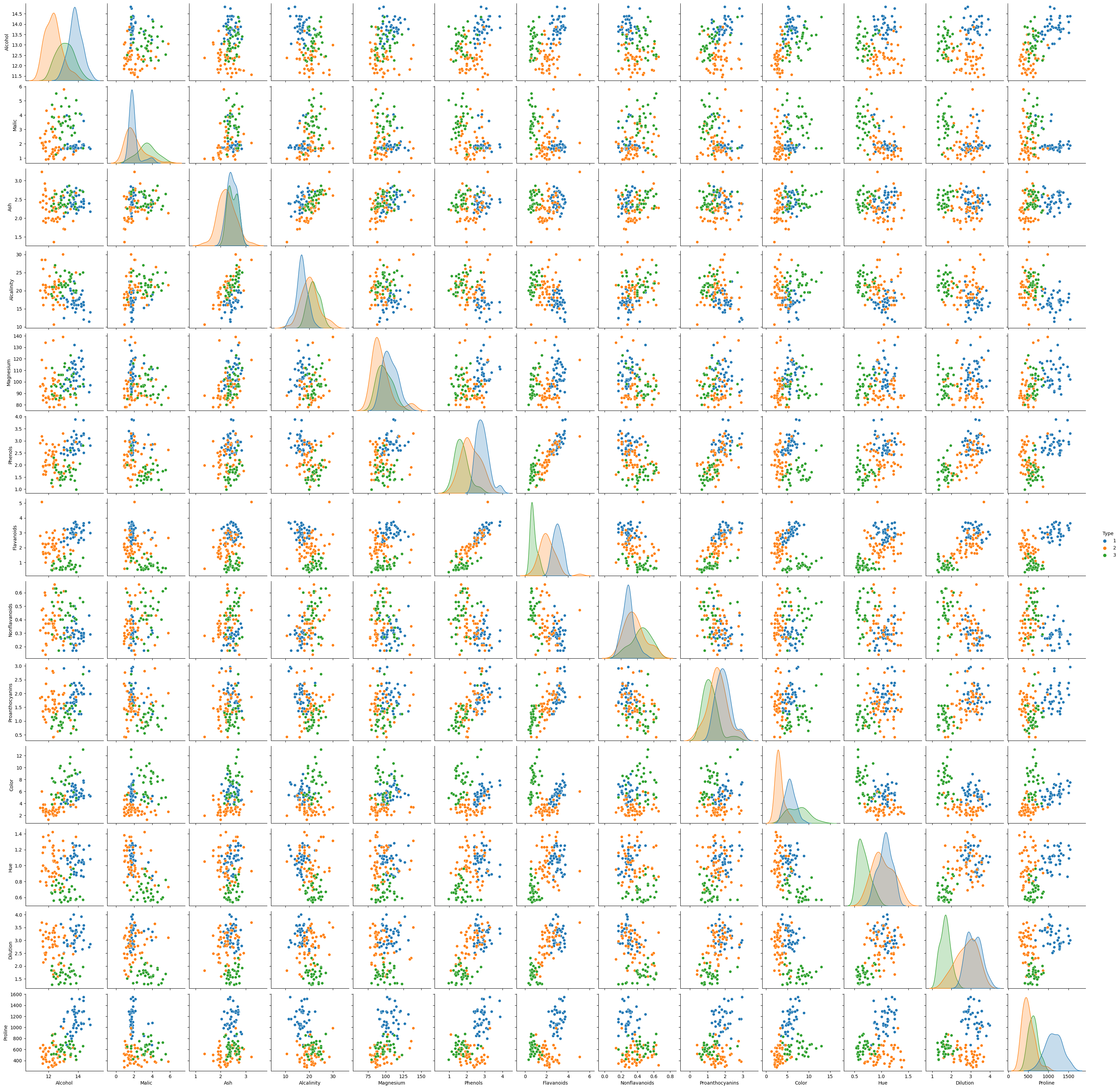
It is hard to see scatter plots because there are so many variables, so let’s focus on several variables. Especially Flavanoids and Color variables seem to be important to classify Type.
fig, axes = plt.subplots(3, 4, figsize = (15, 10))

column_list = ['Alcohol', 'Malic', 'Ash', 'Alcalinity', 'Magnesium', 'Phenols',
               'Nonflavanoids', 'Proanthocyanins', 'Color', 'Hue',
               'Dilution', 'Proline']

for i, col in enumerate(column_list):
    sns.scatterplot(df_train, x = col, y = "Flavanoids", hue = "Type", ax = axes[i // 4, i % 4])

plt.tight_layout()
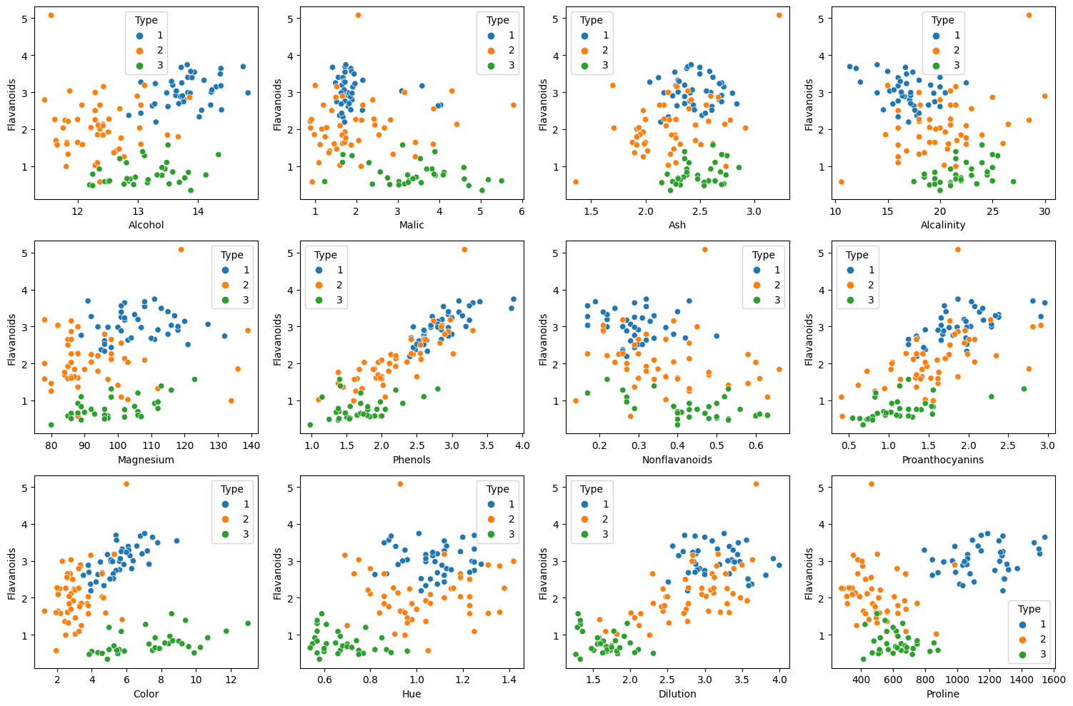
Above plots are scatter plots of Flavanoids with other variables.
- We can easily classify types in almost every scaater plots.
- Especially in scatter plots with Color or Proline, classifying types are more easier.
fig, axes = plt.subplots(3, 4, figsize = (15, 10))

column_list = ['Alcohol', 'Malic', 'Ash', 'Alcalinity', 'Magnesium', 'Phenols',
               'Nonflavanoids', 'Proanthocyanins', 'Flavanoids', 'Hue',
               'Dilution', 'Proline']

for i, col in enumerate(column_list):
    sns.scatterplot(df_train, x = col, y = "Color", hue = "Type", ax = axes[i // 4, i % 4])

plt.tight_layout()
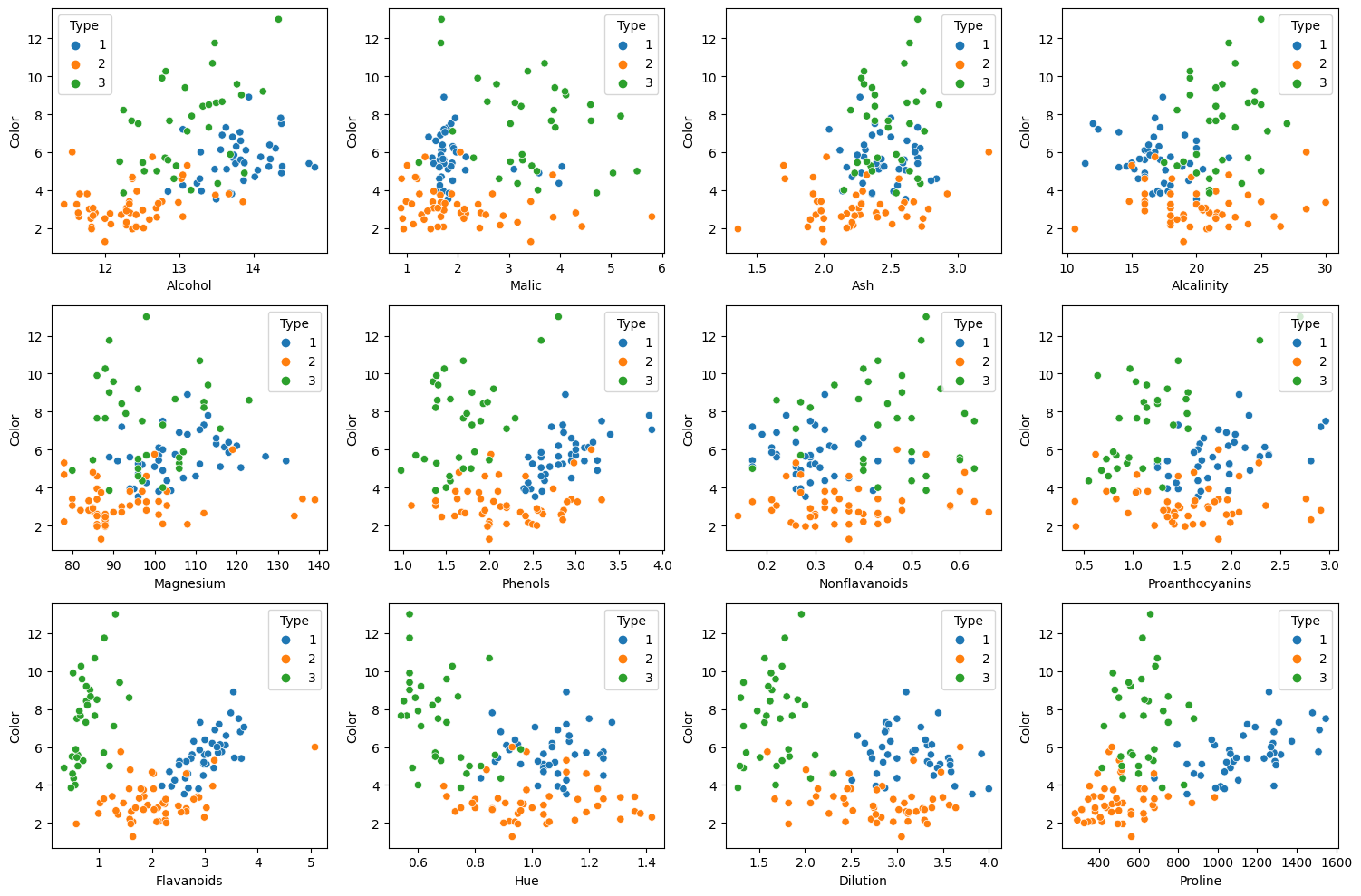
Above plots are scatter plots of Color with other variables.
- In scatter plots with Flavanoids, Proline, or Dilution, we can easily classify types.
fig, axes = plt.subplots(3, 5, figsize = (15, 10))

column_list = ['Alcohol', 'Malic', 'Ash', 'Alcalinity', 'Magnesium', 'Phenols',
               'Flavanoids', 'Nonflavanoids', 'Proanthocyanins', 'Color', 'Hue',
               'Dilution', 'Proline']

for i, col in enumerate(column_list):
    sns.boxplot(df_train, x = "Type", y = col, ax = axes[i // 5, i % 5])

plt.tight_layout()
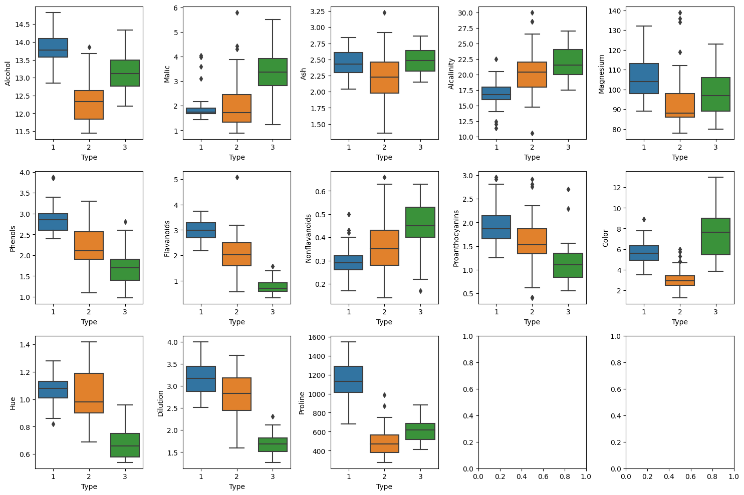
If we check the boxplot, it is more easier to understand wich variables are important for classyfing the Type than the scatter plot. We can see the clear distributional differences between each types in Alchol, Phenols, Flavanoids, Proanthocyanins and Color variables.
(b) Modeling
Perform LDA, QDA and Naive Bayes on the training data in order to predict Type. What are the test errors of the models obtained?
X_train = df_train.drop(["Type"], axis = 1)
y_train = df_train["Type"]
X_test = df_test.drop(["Type"], axis = 1)
y_test = df_test["Type"]
LDA
model_lda = LinearDiscriminantAnalysis()
model_lda.fit(X_train, y_train)
LinearDiscriminantAnalysis()
y_train_pred_lda = model_lda.predict(X_train)
train_error_lda = np.mean(y_train_pred_lda != y_train)

y_test_pred_lda = model_lda.predict(X_test)
test_error_lda = np.mean(y_test_pred_lda != y_test)

print("Train error of LDA: ", train_error_lda)
print("Test error of LDA: ", test_error_lda)
Train error of LDA:  0.0
Test error of LDA:  0.01818181818181818
Train error of LDA is 0.0 but test error of LDA is 0.018.
cm_test_lda = confusion_matrix(y_test, y_test_pred_lda)
cm_display = ConfusionMatrixDisplay(confusion_matrix = cm_test_lda, display_labels = model_lda.classes_)
cm_display.plot()
<sklearn.metrics._plot.confusion_matrix.ConfusionMatrixDisplay at 0x7fbea0fcc6d8>
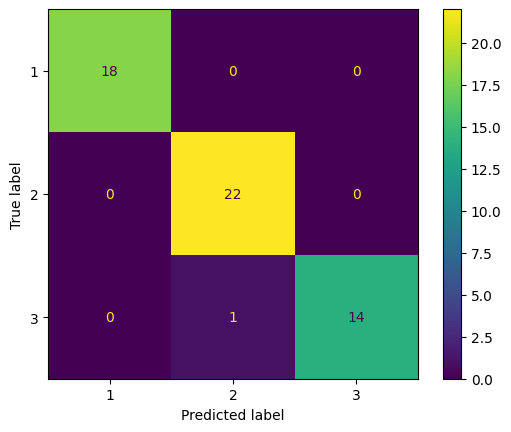
Only one data from type 3 is miss classified to type 2.
X_train_lda = model_lda.transform(X_train)

plt.figure()
colors = ['red', 'green', 'blue']
for color, class_name in zip(colors, model_lda.classes_):
    plt.scatter(X_train_lda[np.array(y_train == class_name).astype("bool"), 0], X_train_lda[np.array(y_train == class_name).astype("bool"), 1],
                alpha=.8, color=color,label= f"Type: {class_name}")
plt.legend(loc='best')
plt.xlabel("LD1")
plt.ylabel("LD2")
plt.show()
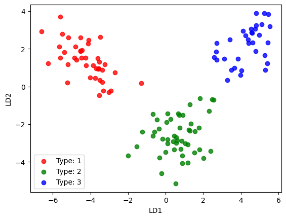
We can see that data points that projected to 2d plane by LDA are well separated between types.
QDA
model_qda = QuadraticDiscriminantAnalysis()
model_qda.fit(X_train, y_train)
QuadraticDiscriminantAnalysis()
y_train_pred_qda = model_qda.predict(X_train)
train_error_qda = np.mean(y_train_pred_qda != y_train)

y_test_pred_qda = model_qda.predict(X_test)
test_error_qda = np.mean(y_test_pred_qda != y_test)

print("Train error of QDA: ", train_error_qda)
print("Test error of QDA: ", test_error_qda)
Train error of QDA:  0.0
Test error of QDA:  0.03636363636363636
Train error of QDA is 0.0 but test error of QDA is 0.036, higher than LDA.
cm_test_qda = confusion_matrix(y_test, y_test_pred_qda)
cm_display = ConfusionMatrixDisplay(confusion_matrix = cm_test_qda, display_labels = model_qda.classes_)
cm_display.plot()
<sklearn.metrics._plot.confusion_matrix.ConfusionMatrixDisplay at 0x7fbec0168828>
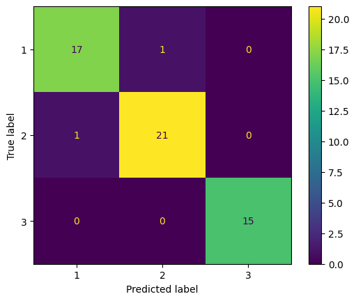
One data from Type 1 is miss classifeid to Type 2, and one data from Type 2 is miss classified to Type 1.
Naive Bayes
model_nb = GaussianNB()
model_nb.fit(X_train, y_train)
GaussianNB()
y_train_pred_nb = model_nb.predict(X_train)
train_error_nb = np.mean(y_train_pred_nb != y_train)

y_test_pred_nb = model_nb.predict(X_test)
test_error_nb = np.mean(y_test_pred_nb != y_test)

print("Train error of Naive Bayes: ", train_error_nb)
print("Test error of Naive Bayes: ", test_error_nb)
Train error of Naive Bayes:  0.016260162601626018
Test error of Naive Bayes:  0.03636363636363636
- Train error is 0.016, higher than LDA and QDA.
- Test error is 0.036, higher than LDA and same with QDA.
cm_test_nb = confusion_matrix(y_test, y_test_pred_nb)
cm_display = ConfusionMatrixDisplay(confusion_matrix = cm_test_nb, display_labels = model_qda.classes_)
cm_display.plot()
<sklearn.metrics._plot.confusion_matrix.ConfusionMatrixDisplay at 0x7fbebf5bcb00>
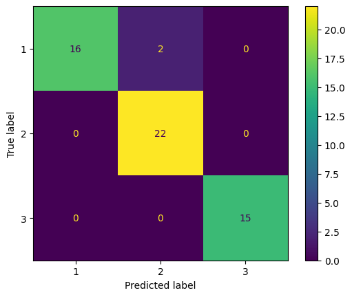
2 data from Type 1 are miss classified to Type 2.
Compare the results
train_error = [train_error_lda, train_error_qda, train_error_nb]
test_error = [test_error_lda, test_error_qda, test_error_nb]

pd.DataFrame({"Train Error" : train_error,
             "Test Error" : test_error}, index = ["LDA", "QDA", "Naive Bayes"])
| Train Error | Test Error | |
|---|---|---|
| LDA | 0.00000 | 0.018182 |
| QDA | 0.00000 | 0.036364 |
| Naive Bayes | 0.01626 | 0.036364 |
- Train error is 0 for both LDA and QDA. Train error of Naive Bayes is 0.016.
- Test error of LDA is the lowest among three methods, 0.018. QDA and Naive Bayes have same test error, 0.036.