
HW3. KNN, Logistic regression
Topics: EDA(Exploratory Data Analysis), KNN, Logistic regression, LOOCV(Leave One Out Cross Validation)
import pandas as pd
import numpy as np
import matplotlib.pyplot as plt
import seaborn as sns
import plotly.express as px
from sklearn.model_selection import train_test_split, KFold, cross_val_score, LeaveOneOut
from sklearn.preprocessing import StandardScaler
from sklearn.neighbors import KNeighborsClassifier
import matplotlib.patches as mpatches
from sklearn.linear_model import LogisticRegression
from sklearn.metrics import confusion_matrix, ConfusionMatrixDisplay
import warnings
warnings.filterwarnings('ignore')
Problem 1: Theft dataset
Use thek-nearest neighbor classifier on the Theft dataset. Use cross-validation to select the best k and use the test data to evaluate the performance of the selected model. Show the training, cross- validation and test errors for each choice of k and report your findings.
1.1. EDA
About data
theft_train = pd.read_csv("theft_train.csv")
theft_test = pd.read_csv("theft_test.csv")
theft_train.head()
| X | Y | theft | hour | |
|---|---|---|---|---|
| 0 | -122.390434 | 37.750118 | False | 9 |
| 1 | -122.404452 | 37.800802 | True | 18 |
| 2 | -122.412447 | 37.775634 | False | 18 |
| 3 | -122.419695 | 37.789777 | True | 4 |
| 4 | -122.406725 | 37.758564 | False | 16 |
theft_train.dtypes
X        float64
Y        float64
theft       bool
hour       int64
dtype: object
theft_train.describe()
| X | Y | hour | |
|---|---|---|---|
| count | 3500.000000 | 3500.000000 | 3500.000000 |
| mean | -122.422842 | 37.770337 | 13.858286 |
| std | 0.024839 | 0.022981 | 6.205993 |
| min | -122.513642 | 37.708311 | 0.000000 |
| 25% | -122.432742 | 37.759719 | 10.000000 |
| 50% | -122.416823 | 37.776799 | 15.000000 |
| 75% | -122.407151 | 37.785684 | 19.000000 |
| max | -122.364937 | 37.810204 | 23.000000 |
theft_test.describe()
| X | Y | hour | |
|---|---|---|---|
| count | 1500.000000 | 1500.000000 | 1500.000000 |
| mean | -122.422429 | 37.769261 | 13.946667 |
| std | 0.024695 | 0.023764 | 6.358205 |
| min | -122.511294 | 37.708995 | 0.000000 |
| 25% | -122.432006 | 37.755804 | 10.000000 |
| 50% | -122.416284 | 37.775740 | 15.000000 |
| 75% | -122.406543 | 37.785957 | 19.000000 |
| max | -122.365565 | 37.809671 | 23.000000 |
- X: longitude. Only have negative float values.
- Y: Latitude. Only have positive float values.
- hour: Timestamp of the crime incident. Only have positive integer values range 0 ~ 24.
- theft: Class variable (0 or 1). 1 if larcency/theft, 0 otherwise
print("train data shape: ", theft_train.shape)
print("test data shape: ", theft_test.shape)
train data shape:  (3500, 4)
test data shape:  (1500, 4)
There are 3500 data for training set, 1500 data for test set.
Missing values
theft_train.isna().sum()
X        0
Y        0
theft    0
hour     0
dtype: int64
theft_test.isna().sum()
X        0
Y        0
theft    0
hour     0
dtype: int64
There are no missing values.
Dependent variables
sns.countplot(theft_train, x = "theft")
<Axes: xlabel='theft', ylabel='count'>
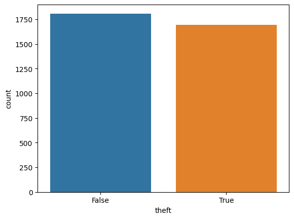
True and False from “theft” variable are equally distributed.
Independent variables
hour
sns.histplot(theft_train, x = "hour")
<Axes: xlabel='hour', ylabel='Count'>
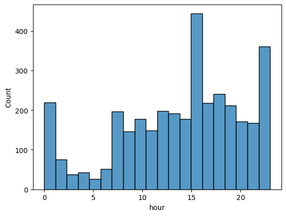
- Crime rarely occurs in the early morning hours, and increases in the afternoon hours.
- Crime is most common around 6pm or 11pm.
- However, we need to check whether theft crime and other crimes show different time distributions.
hour ~ theft
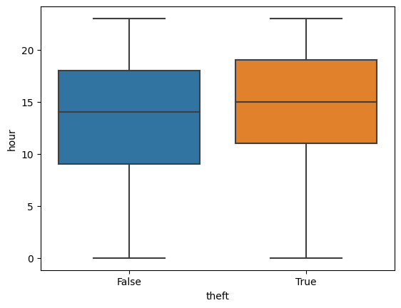
Hypothesis: There are some time range that theft crimes are common.
sns.boxplot(theft_train, x = "theft", y = "hour")
<Axes: xlabel='theft', ylabel='hour'>
sns.histplot(theft_train, x = "hour", hue = "theft")
<AxesSubplot:xlabel='hour', ylabel='Count'>
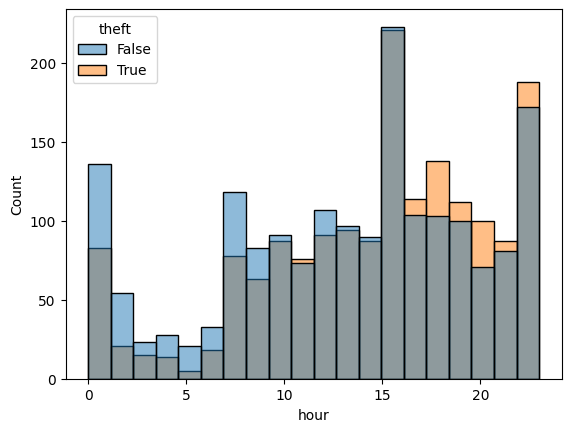
Theft crimes and other crimes have same time ditributions. Therefore, we can say that there are no time range that theft crime common.
location ~ theft
Hypothesis: There are specific locations where theft crimes are common.
sns.scatterplot(theft_train, x = "X", y = "Y", hue = "theft", alpha = 0.5)
<Axes: xlabel='X', ylabel='Y'>
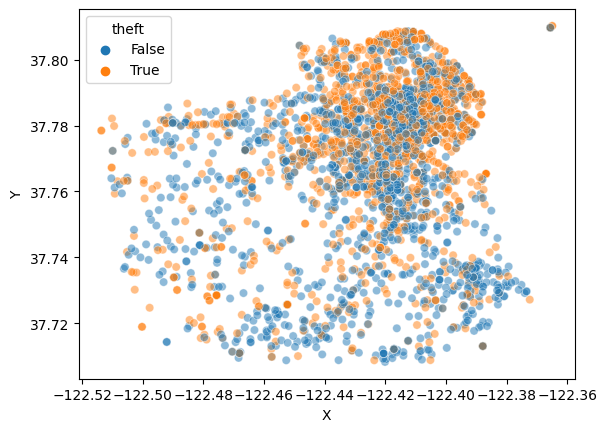
- We can see that there are more cirmes in the northeast area than other areas.
- It looks like that some parts of the northeast have more theft crimes.
1.2. Modeling: KNN
Let’s compare result of knn that depends on the neighbor numbers K = 1, …, 150. I used 5-fold cross validation to compare the result.
theft_kf = KFold(n_splits = 5)

n_neighbors_list = np.arange(1, 151)
train_error_list = []
cv_error_list = []
test_error_list = []

for n_neighbors in n_neighbors_list:
    ## calculate k-fold cv error
    cv_error = []

    for i, (train_index, valid_index) in enumerate(theft_kf.split(theft_train)):
        x_train = theft_train.iloc[train_index].drop("theft", axis = 1)
        y_train = theft_train.iloc[train_index]["theft"]

        x_valid = theft_train.iloc[valid_index].drop("theft", axis = 1)
        y_valid = theft_train.iloc[valid_index]["theft"]

        scaler = StandardScaler()
        scaler.fit(x_train)

        x_train_std = scaler.transform(x_train)
        x_valid_std = scaler.transform(x_valid)

        knn = KNeighborsClassifier(n_neighbors = n_neighbors)
        knn.fit(x_train_std, y_train)
        pred_val = knn.predict(x_valid_std)

        cv_error.append(np.mean(pred_val != y_valid))

    cv_error_list.append(np.mean(cv_error))

    ## calculate train, test error
    x_train = theft_train.drop("theft", axis = 1)
    y_train = theft_train["theft"]

    x_test = theft_test.drop("theft", axis = 1)
    y_test = theft_test["theft"]

    scaler = StandardScaler()
    scaler.fit(x_train)

    x_train_std = scaler.transform(x_train)
    x_test_std = scaler.transform(x_test)

    knn = KNeighborsClassifier(n_neighbors = n_neighbors)
    knn.fit(x_train_std, y_train)
    pred_train = knn.predict(x_train_std)
    pred_test = knn.predict(x_test_std)

    train_error_list.append(np.mean(pred_train != y_train))
    test_error_list.append(np.mean(pred_test != y_test))
plt.grid()
sns.lineplot(x = 1/n_neighbors_list, y = cv_error_list, color = "blue")
sns.lineplot(x = 1/n_neighbors_list, y = train_error_list, color = "green")
sns.lineplot(x = 1/n_neighbors_list, y = test_error_list, color = "red")
plt.xlabel("Number of neighbors (1 / k)")
plt.ylabel("Error")
plt.title("5-fold errors with different choice of neighbor k for KNN")

train_error = mpatches.Patch(color = "green", label = "Train error")
test_error = mpatches.Patch(color = "red", label = "Test error")
validation_error = mpatches.Patch(color = "blue", label = "Validation error")
plt.legend(handles = [train_error, test_error, validation_error])
<matplotlib.legend.Legend at 0x7ff690ef5dd8>
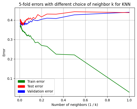
- We can check that the more complex the model, the smaller the train error.
- As the model becomes more complex, the test error and validation error decrease and then increase again.
best_k_indx = np.argmin(cv_error_list)
print("Best number of neighbor k: ", n_neighbors_list[best_k_indx])
print("Train error at best k: ", train_error_list[best_k_indx])
print("Validation error at best k: ", cv_error_list[best_k_indx])
print("Test error at best k: ", test_error_list[best_k_indx])
Best number of neighbor k:  37
Train error at best k:  0.3442857142857143
Validation error at best k:  0.372
Test error at best k:  0.378
Problem 2: Weekly dataset
2.1. EDA
About data
weekly = pd.read_csv("Weekly_Data.csv", index_col = 0).reset_index().drop("index", axis = 1)
weekly.head()
| Year | Lag1 | Lag2 | Lag3 | Lag4 | Lag5 | Volume | Today | Direction | |
|---|---|---|---|---|---|---|---|---|---|
| 0 | 1990 | 0.816 | 1.572 | -3.936 | -0.229 | -3.484 | 0.154976 | -0.270 | Down |
| 1 | 1990 | -0.270 | 0.816 | 1.572 | -3.936 | -0.229 | 0.148574 | -2.576 | Down |
| 2 | 1990 | -2.576 | -0.270 | 0.816 | 1.572 | -3.936 | 0.159837 | 3.514 | Up |
| 3 | 1990 | 3.514 | -2.576 | -0.270 | 0.816 | 1.572 | 0.161630 | 0.712 | Up |
| 4 | 1990 | 0.712 | 3.514 | -2.576 | -0.270 | 0.816 | 0.153728 | 1.178 | Up |
weekly.dtypes
Year           int64
Lag1         float64
Lag2         float64
Lag3         float64
Lag4         float64
Lag5         float64
Volume       float64
Today        float64
Direction     object
dtype: object
This data is about weekly percentage returns for the S&P 500 stock index between 1990 and 2010.
All variables are numerical variables except for Direction.
- Year: the year that the observation was recorded
- Lag n: percentage return for n weeks previous
- Volumne: volume of shares traded (average number of daily shares traded in billions)
- Today: percentage return for this week
- Direction: a factor with levels Down and Up indicating whether the market had a positive or negative return on a given week
weekly.shape
(1089, 9)
There are 1089 observations.
Missing values
weekly.isna().sum()
Year         0
Lag1         0
Lag2         0
Lag3         0
Lag4         0
Lag5         0
Volume       0
Today        0
Direction    0
dtype: int64
There is no missing value.
Dependent varaible
sns.countplot(weekly, x = "Direction")
<Axes: xlabel='Direction', ylabel='count'>
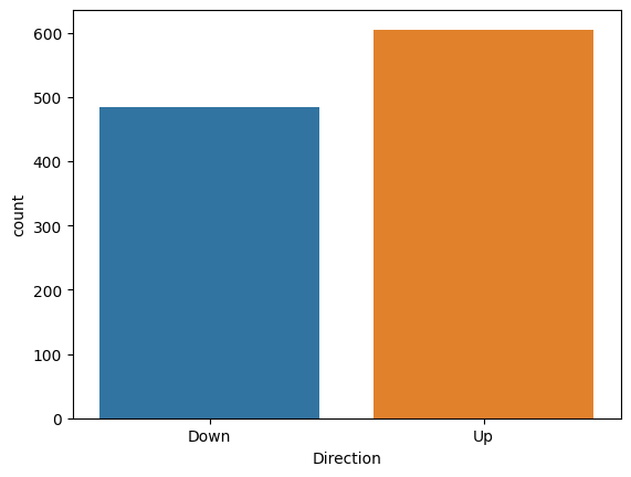
The number of up and down are almost evenly distributed.
Independent variables
Year
plt.figure(figsize = (15, 5))
sns.countplot(weekly, x = "Year")
<Axes: xlabel='Year', ylabel='count'>
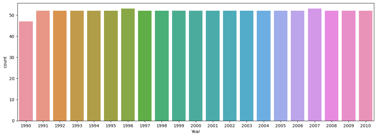
There are 52 or 53 weeks for each year except for 1990 year.
Today
weekly.Today.describe()
count    1089.000000
mean        0.149899
std         2.356927
min       -18.195000
25%        -1.154000
50%         0.241000
75%         1.405000
max        12.026000
Name: Today, dtype: float64
fig, (ax_box, ax_hist) = plt.subplots(2, sharex = True, gridspec_kw = {"height_ratios": (.2, .8)}, figsize = (10, 7))

sns.boxplot(x = weekly.Today, ax = ax_box, showfliers = False)
sns.histplot(x = weekly.Today, ax = ax_hist, kde = True)

plt.xlabel("Percentage return for this week (Today)", fontsize = 16)
plt.ylabel("Count", fontsize = 16)
ax_box.set_xlabel("")

plt.show()
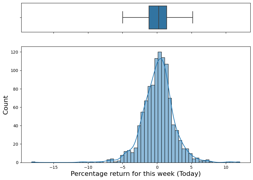
Percentage return for this week almost follows noirmal distribution with mean = 0.24.
Today ~ Direction
sns.histplot(weekly, x = "Today", hue = "Direction")
<Axes: xlabel='Today', ylabel='Count'>
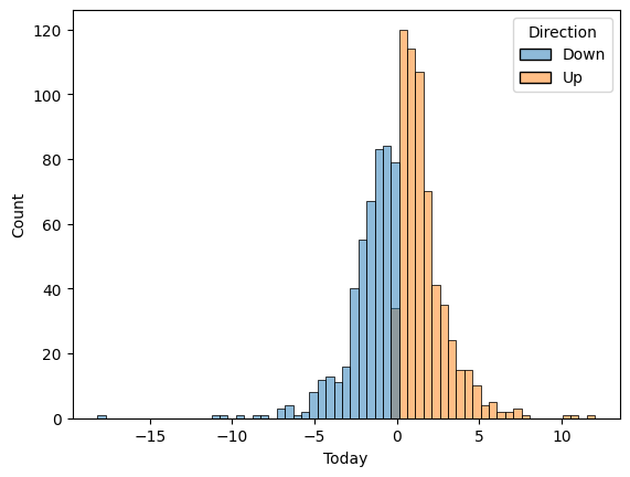
weekly[weekly["Today"] < 0].Direction.value_counts()
Down    484
Name: Direction, dtype: int64
weekly[weekly["Today"] > 0].Direction.value_counts()
Up    605
Name: Direction, dtype: int64
Since Today variable means the percentage return for this week and Direction variable indicates direction of this week, they have the same direction.
Volume
weekly.Volume.describe()
count    1089.000000
mean        1.574618
std         1.686636
min         0.087465
25%         0.332022
50%         1.002680
75%         2.053727
max         9.328214
Name: Volume, dtype: float64
fig, (ax_box, ax_hist) = plt.subplots(2, sharex = True, gridspec_kw = {"height_ratios": (.2, .8)}, figsize = (10, 7))

sns.boxplot(x = weekly.Volume, ax = ax_box, showfliers = False)
sns.histplot(x = weekly.Volume, ax = ax_hist, kde = True)

plt.xlabel("Volume of shares traded", fontsize = 16)
plt.ylabel("Count", fontsize = 16)
ax_box.set_xlabel("")

plt.show()
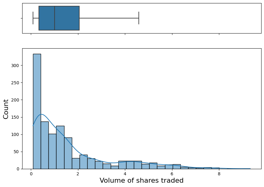
The volume variable has range (0.087, 9.328). The mean is 1.57 and the median is 1.00. The Volume variable has a long tail distribution.
Volume ~ Direction
sns.histplot(weekly, x = "Volume", hue = "Direction")
<Axes: xlabel='Volume', ylabel='Count'>
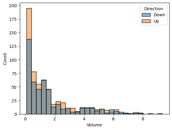
Volumes with Up direction and Volumes with Down direction have almost same ditributions.
Volume ~ Year
sns.scatterplot(weekly, x = "Year", y = "Volume", hue = "Direction")
<Axes: xlabel='Year', ylabel='Volume'>
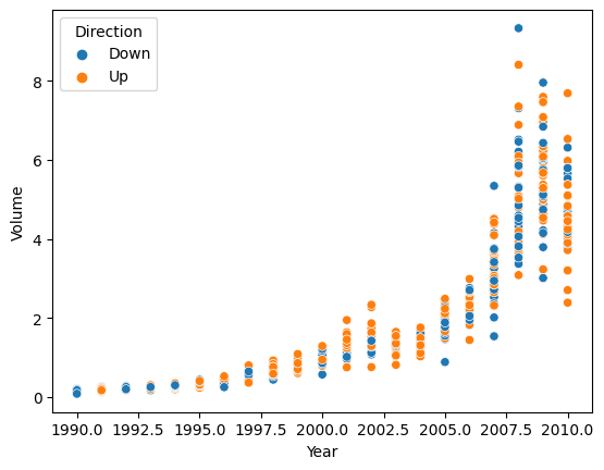
As time passes, the value of volume increases and the range also gradually widens. However, there is no clear relationship with Direction.
Lag1, Lag2
fig, ((ax_box1, ax_box2),
      (ax_hist1, ax_hist2)) = plt.subplots(2, 2, sharex = True,
                                           gridspec_kw = {"height_ratios": (.2, .8)}, figsize = (10, 7))

sns.boxplot(x = weekly.Lag1, ax = ax_box1, showfliers = False)
sns.histplot(x = weekly.Lag1, ax = ax_hist1, kde = True)

ax_hist1.set_xlabel("Percentage return for previous week", fontsize = 12)
ax_hist1.set_ylabel("Count", fontsize = 12)
ax_box1.set_xlabel("")

sns.boxplot(x = weekly.Lag2, ax = ax_box2, showfliers = False)
sns.histplot(x = weekly.Lag2, ax = ax_hist2, kde = True)

ax_hist2.set_xlabel("Percentage return for 2 weeks previous", fontsize = 12)
ax_hist2.set_ylabel("Count", fontsize = 12)
ax_box2.set_xlabel("")

plt.show()
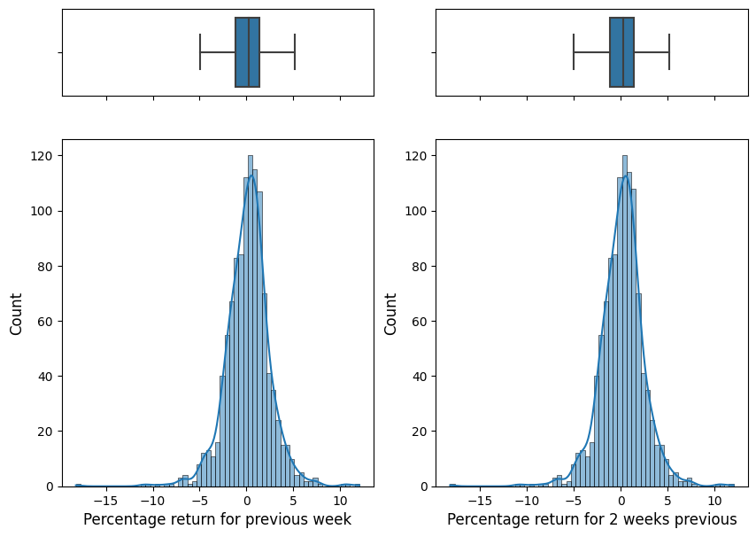
Lag1 and Lag2 follow almost same distribution.
Lag1, Lag2 ~ Today
fig, axes = plt.subplots(1, 2, figsize = (15, 5))

sns.scatterplot(weekly, x = "Lag1", y = "Today", hue = "Direction", ax = axes[0])
sns.scatterplot(weekly, x = "Lag2", y = "Today", hue = "Direction", ax = axes[1])
axes[0].grid()
axes[1].grid()
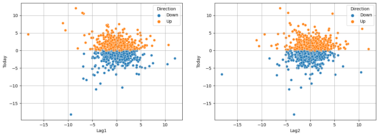
It looks like that there are no relationship between percentage return for this week and previous week or 2 weeks previous.
Corelation
corr = weekly.corr()
mask = np.triu(np.ones_like(corr, dtype=bool))

sns.heatmap(corr, mask = mask, annot = True, cmap = "BrBG", vmin = -1, vmax = 1,
            linewidths = 0.5, cbar_kws = {"shrink" : 0.5})
/var/folders/kb/9bgdwxjn0b751yc9w59v1ll00000gn/T/ipykernel_7344/2939553793.py:1: FutureWarning:

The default value of numeric_only in DataFrame.corr is deprecated. In a future version, it will default to False. Select only valid columns or specify the value of numeric_only to silence this warning.


<Axes: >
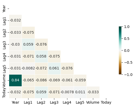
There is no clear correlation between variables except for Year and Volume.
2.2. Modeling: Logistic regression
(2.2.a)
Fit a logistic regression model that predicts Direction using Lag1 and Lag2. Report and comment on the result.
logit_model = LogisticRegression()
logit_model.fit(weekly[["Lag1", "Lag2"]], weekly["Direction"])
pred = logit_model.predict(weekly[["Lag1", "Lag2"]])
np.mean(pred != weekly.Direction)
0.44536271808999084
Classification error is 0.445
cm = confusion_matrix(weekly.Direction, pred)
cm_display = ConfusionMatrixDisplay(confusion_matrix = cm, display_labels = logit_model.classes_)
cm_display.plot()
<sklearn.metrics._plot.confusion_matrix.ConfusionMatrixDisplay at 0x7fd27b6d68f0>
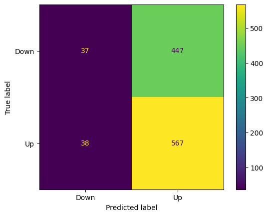
- 447 cases out of 484 cases are missclassified to Up.
- 38 cases out of 605 cases are missclassified to Down.
(2.2.b)
Fit a logistic regression model that predicts Direction using Lag1 and Lag2 using all but the first observation. Report and comment on the result.
X = weekly[["Lag1", "Lag2"]]
y = weekly.Direction
X = weekly[["Lag1", "Lag2"]]
y = weekly.Direction

X_train = X.drop(0)
y_train = y.drop(0)
X_valid = np.array(X.iloc[0]).reshape(1, -1)
y_valid = y.iloc[0, ]
logit_model = LogisticRegression()
logit_model.fit(X_train, y_train)
pred = logit_model.predict(X_train)
np.mean(pred != y_train)
0.4430147058823529
Classification error for the data except for the first observation is 0.443. This error means one of training errors of LOOCV.
(2.2.c)
| Use the model from(b) to predict the direction of the first observation. You can do this by predicting that the first observation will go up if Pr(Direction=“Up” | Lag1, Lag2) > 0.5. Was this observation correctly classified? |
logit_model.predict_proba(X_valid)
/Users/youngjun/anaconda3/envs/data_analysis_venv/lib/python3.10/site-packages/sklearn/base.py:420: UserWarning:

X does not have valid feature names, but LogisticRegression was fitted with feature names


array([[0.42861856, 0.57138144]])
logit_model.classes_
array(['Down', 'Up'], dtype=object)
| The second class is the direction Up. Since $P(Direction = “Up” | Lag1, Lag2) = 0.57 > 0.5$, we can predict the direction will be Up. |
y_valid
'Down'
Since the true direction is Down, this observation is not correctly classified.
(2.2.d)
Writea for loop from i=1 to i=n, where n is the numberof observations in the data set, that performs each of the following steps:
1) Fit a logistic regression model using all but the ith observation to predict Direction using Lag1 and Lag2.
2) Compute the posterior probability of the market moving up for the ith observation.
3) Use the posterior probability for the ith observation in order to predict whether or not the market moves up.
4) Determine whether or not an error was made in predicting the direction for the ith observation. If an error was made, then indicate this as a 1, and otherwise indicate it as a 0.
X = weekly[["Lag1", "Lag2"]]
y = weekly.Direction

n = weekly.shape[0]

error_list = []
for i in range(n):
    # Set ith observation as validation data, all others as train data
    X_train = X.drop(i)
    y_train = y.drop(i)
    X_valid = np.array(X.iloc[i]).reshape(1, -1)
    y_valid = y.iloc[i, ]

    # Fit a logistic regression model using all but the ith observation to predict Direction using Lag1 and Lag2
    logit_model = LogisticRegression()
    logit_model.fit(X_train, y_train)

    # Compute the posterior probability of the market moving up for the ith observation
    pred_prob = logit_model.predict_proba(X_valid)

    # Use the posteriro probability for the ith observation in order to predict wheter or not the market moves up
    up_prob = logit_model.predict_proba(X_valid)[0][logit_model.classes_ == "Up"]
    if up_prob >= 0.5: pred = "Up"
    else: pred = "Down"

    # Determine wheter or not an error was made in predicting the direction for the ith observation.
    # If an error was made, then indicate this as a 1, and otherwise indicate it as a 0
    if y_valid != pred: error = 1
    else: error = 0

    error_list.append(error)
(2.2.e)
Take the average of the n numbers obtained in (d)iv in order to obtain the LOOCV estimate for the test error. Comment on the results.
np.mean(error_list)
0.44995408631772266
LOOCV estimate for the test error is 0.449. This error is bigger than the error from (a) and (b), where we fitted models and got errors from the fitted training data.