HW1

22 minute read

Topics: Return, Log return, ACF(Auto Correlation Function), QQ plot, VaR(Value at Risk), Coupon bond

Problem 1

(1. a)

Read the tutorial on accessing and downloading data from WRDS available on this link.

(1. b)

Execute a query to download the closing daily prices of the stocks with tickers TSLA and AAPL for the period Jan 1, 2022 through Jan 6, 2023.

(1. c)

Place the resulting CSV file in a desired folder in your computer and modify the following code to produce plots of daily prices, returns, log-returns, and a scatter-plot of the log-returns of TSLA against those of AAPL. Identify the times of splits if any for the AAPL and TSLA stock in this period.

Solution

dat = read.csv("data/aapl_tsla_daily.csv",header=TRUE)

t <- as.Date(as.character(dat$date), "%Y%m%d")

stock_tickers = unique(dat$TICKER)
stocks = list("AAPL" = c(), "TSLA" = c())
times = stocks
R = stocks
r = stocks

for (tick in stock_tickers){
    idx_tick = which(dat$TICKER == tick)
    idx_prc = which((is.na(dat$PRC[idx_tick]) == FALSE) &
                    (dat$PRC[idx_tick] >= 0))
    times[[tick]] = t[idx_tick[idx_prc]]
    stocks[[tick]] = abs(dat$PRC[idx_tick[idx_prc]])
    n = length(stocks[[tick]])
    R[[tick]] = stocks[[tick]][-1] / stocks[[tick]][-n] - 1
    r[[tick]] = diff(log(stocks[[tick]]))
}

## AAPL ###
options(repr.plot.width=15, repr.plot.height=15)
par(mfrow = c(2,2))
plot(times$AAPL, stocks$AAPL, type = "l",
     xlab = "Time (days)", ylab = "USD",
     main = "Daily Stock Prices: AAPL")
plot(times$AAPL[-1], 100 * R$AAPL, type = "l",
     xlab = "Time (days)", ylab = "Daily return (%)",
     main = paste("Returns for AAPL: n = ", n, "days"))
plot(times$AAPL[-1], 100 * r$AAPL, type = "l",
     xlab = "Time (days)", ylab = "Daily log-return (%)",
     main = paste("Log-returns for AAPL: n = ", n, "days"))
plot(100 * r$AAPL, 100 * r$TSLA,
     xlab = "Daily log-return (%) of AAPL", ylab = "Daily log-return (%) of TSLA",
     main = "Log-returns of AAPl vs TSLA")

png

### TSLA ###
options(repr.plot.width=15, repr.plot.height=15)
par(mfrow = c(2,2))
plot(times$TSLA, stocks$TSLA, type = "l",
     xlab = "Time (days)", ylab = "USD",
     main = "Daily Stock Prices: TSLA")
plot(times$TSLA[-1], 100 * R$TSLA, type = "l",
     xlab = "Time (days)", ylab = "Daily return (%)",
     main = paste("Returns for TSLA: n = ", n, "days"))
plot(times$TSLA[-1], 100 * r$TSLA, type = "l",
     xlab = "Time (days)", ylab = "Daily log-return (%)",
     main = paste("Log-returns for TSLA: n = ", n, "days"))
plot(100 * r$AAPL, 100 * r$TSLA,
     xlab = "Daily log-return (%) of AAPL", ylab = "Daily log-return (%) of TSLA",
     main = "Log-returns of AAPl vs TSLA")

png

Problem 2

Download the file ”sp500 full.csv” available in the Data folder of the Files section in Canvas. It provides the data on daily prices and returns (among other things) of the S&P 500 index. This is the same data set used in lectures.

(2. a)

Plot the time-series of daily returns and daily log-returns. You need to identify which variable gives the returns and also compute the log-returns from the daily closing values of the index. Comment on the extreme drops in daily returns/log-returns. Can they be associated with known market events?

Solution

sp = read.csv("data/sp500_full.csv")

sp.t = as.Date(as.character(sp$caldt), format = "%Y%m%d")
idx = which(sp.t >= "1960-01-01")
sp.t = sp.t[idx]

sp.price = sp$usdval[idx]

n = length(sp.price)
sp.return = sp.price[-1] / sp.price[-n] - 1
sp.log_return = diff(log(sp.price))

options(repr.plot.width=15, repr.plot.height=8)
par(mfrow = c(1, 2))

plot(sp.t[-1], 100 * sp.return, type = "l",
     xlab = "Time (days)", ylab = "Daily return (%)",
     main = "Daily returns of SP500")
plot(sp.t[-1], 100 * sp.log_return, type = "l",
     xlab = "Time (days)", ylab = "Daily log-return (%)",
     main = "Daily log-returns of SP500")

png

We can check large drop of daily returns and daily log-returns on 1980 1990, which may be related to Black Monday.
We can check large drops of daily returns and daily log-returns on about 2000, which may be related to collapse of Dot-com bubble.
We can check large drops of daily returns and daily log-returns on about 2010, which may be related to Sub-prime mortgage meltdown.
We can check large drops of daily returns and daily log-returns on about 2020, which may be related to COVID-19.

(2. b)

Plot the auto-correlation functions of the 1-day (i.e., daily), 5-day, 10-day and 20-day log-returns and their squares.

Solution

options(repr.plot.width=15, repr.plot.height=15)

sp.log_return_5 = diff(log(sp.price), 5)
sp.log_return_10 = diff(log(sp.price), 10)
sp.log_return_20 = diff(log(sp.price), 20)

par(mfrow = c(4, 2))

acf(sp.log_return[sp.log_return >-0.5],
    main = "ACF of the 1-day log-returns")
acf(sp.log_return[sp.log_return >-0.5]^2,
    main = "ACF of the 1-day squared log-returns")

acf(sp.log_return_5[sp.log_return_5 >-0.5],
    main = "ACF of the 5-day log-returns")
acf(sp.log_return_5[sp.log_return_5 >-0.5]^2,
    main = "ACF of the 5-day squared log-returns")

acf(sp.log_return_10[sp.log_return_10 >-0.5],
    main = "ACF of the 10-day log-returns")
acf(sp.log_return_10[sp.log_return_10 >-0.5]^2,
    main = "ACF of the 10-day squared log-returns")

acf(sp.log_return_20[sp.log_return_20 >-0.5],
    main = "ACF of the 20-day log-returns")
acf(sp.log_return_20[sp.log_return_20 >-0.5]^2,
    main = "ACF of the 20-day squared log-returns")

png

(2. c)

Provide a table of the basic summary statistics for the 4 time series from part (b). That is, compute the minimum, 1st quartile, the median, the 3rd quartile and the maximum, for the k-day log-returns for k = 1,5,10, and 20. You can modify the code in the ”.Rnw” file that produces:

Solution

acf_log_returns = list("1d" = sp.log_return, "5d" = sp.log_return_5, 
                       "10d" = sp.log_return_10, "20d" = sp.log_return_20)

acf_summary = lapply(acf_log_returns, summary)

x = matrix(0, nrow = 4, ncol = 6, dimnames = list(c("1-day", "5-day", "10-day", "20-day"), names(acf_summary$`1d`)))
x[1,] = acf_summary$`1d`
x[2,] = acf_summary$`5d`
x[3,] = acf_summary$`10d`
x[4,] = acf_summary$`20d`

x

A matrix: 4 × 6 of type dbl
	Min.	1st Qu.	Median	Mean	3rd Qu.	Max.
1-day	-0.2164902	-0.004171169	0.0005320927	0.0003270746	0.005146278	0.1089740
5-day	-0.3069056	-0.010196493	0.0030848428	0.0016349423	0.014386796	0.1730913
10-day	-0.3665458	-0.012503899	0.0057800224	0.0032692539	0.021055013	0.1934883
20-day	-0.3686597	-0.015743542	0.0108073613	0.0065576122	0.032330457	0.2080365

Problem 3

(3. a)

Using the same data set as in the previous problem, make a 2 × 2 array of normal quantile-quantile plots. You can uncomment and and modify the following code

Solution

options(repr.plot.width=12, repr.plot.height=12)
par(mfrow = c(2,2))
qqnorm(sp.log_return, main = "Normal Q-Q Plot: ACF 1-day")
qqline(sp.log_return, col = "red")
qqnorm(sp.log_return_5, main = "Normal Q-Q Plot: ACF 5-day")
qqline(sp.log_return_5, col = "red")
qqnorm(sp.log_return_10, main = "Normal Q-Q Plot: ACF 10-day")
qqline(sp.log_return_10, col = "red")
qqnorm(sp.log_return_20, main = "Normal Q-Q Plot: ACF 20-day")
qqline(sp.log_return_20, col = "red")

png

(3. b)

What can you say about the tails of the returns?

Solution

Since the right-sides and left-sides of the plot curves up away from the line, the distribution of the all 4 data have heavier right and left tail than the normal distribution. Especially, left side is more heavier than right side. Also we can check that the larger the k-day, the heavier the left-side.

Problem 4

(4. a)

Go to the US Treasury web-site and look up the annual yield to maturity of US government issued zero-coupon bonds of maturities 3 months, 5 years and 30 years, respectively. What are the names of these 3 types of securities?

Solution

3 months (Treasury bills): 4.69
5 years (Treasury notes): 3.43
30 years (Treasury bonds): 3.54

(4. b)

Suppose that a bond with maturity T = 30 years, PAR $1000 and annual coupon payments C is selling precisely at its par value. Determine the value of the coupon payments C. You can assume that the yield to maturity is the one you found in part (a), corresponding to maturity T = 30.

Solution

T = 30
PAR = 1000
V = 1000
r = 3.54 by P4-(a)
Then by the formulation from the lecture, we can calculate C = 35.4

(4. c)

Use the R-function uniroot to find the yield to maturity of a 30-year, par \$1000 bond with annual coupon payments of \$40, which is selling for \$1200 now. Provide the R-code as well as the output.

Solution

find_yield <- function(r, C, PAR, T){
    V = C/r + (PAR - (C / r)) * (1 / (1 + r) ^ T)
    
    return (V)
}

uniroot(function(x, C, PAR, T)(1200 - find_yield(x, C, PAR, T)), 
        interval = c(0.0001, 0.06), C = 40, PAR = 1000, T = 30)$root

0.0297938804894914

The yield to maturity of a 30-year, par \$1000 bond with annual coupon payments of \$40, which is selling for \$1200 now is 0.0297

Problem 5

Suppose (although this is dangerously far from reality) that the daily log-returns of the S&P 500 are independent and identically distributed $N(\mu, \sigma^2)$.

(5. a)

Using the data in file ”sp500 full.csv”, estimate $\mu$ and $\sigma$ with the sample mean and standard deviation.

Solution

mean(sp.log_return)
sd(sp.log_return)

0.000327074561361092

0.0103759072329351

sample mean: 0.00032
sample standard deviation: 0.01

(5. b)

Using the independence and Normality assumptions, compute the value-at-risk at level $\alpha = 0.05$, i.e., $VaR_{0.05}$ for the k-day log-returns, where k = 1, 5, 10 and 20.

Solution

mu = mean(sp.log_return)
sig = sd(sp.log_return)

var = -(mu + sig*qnorm(0.05))
var

0.0167397740836443

k-day log-returns follow same distribution with daily log-returns. So $VaR_{0.05}$ for the k-day log-returns, where k = 1, 5, 10 and 20 are 0.0167.

(5. c)

Provide a table of the proportion of times the k-day log-returns were lower than the $-VaR_{0.05}$ values computed in part (b). That is, the proportion of time the k-day log-losses were worse than the value-at-risk.

Solution

lt_var = c(sum(sp.log_return < -var) / length(sp.log_return),
           sum(sp.log_return_5 < -var) / length(sp.log_return_5),
           sum(sp.log_return_10 < -var) / length(sp.log_return_10),
           sum(sp.log_return_20 < -var) / length(sp.log_return_20))

p = matrix(0,nrow=1,ncol=4,
           dimnames=list("Freq below VaR",
                         c("1-day","5-day","10-day","20-day")))


p[1, ] = lt_var

p

A matrix: 1 × 4 of type dbl
	1-day	5-day	10-day	20-day
Freq below VaR	0.03972831	0.1626074	0.2113868	0.2425098

Problem 6

In this problem we will first find a slightly more appropriate model for the log-returns of the SP500 index data set. The idea is to replace the increments of the normal random walk model in the previous problem with t-distribued increments. We will do so by trial and error and eyeballing QQ-plots. More sophisticated inference methods will come shortly.

(6. a)

As in Problem 2 above, load the SP500 data set from file sp500 full.csv. Select a consecutive period of 10 years. Standardize the log-returns in this period and produce a series of QQ-plots of the daily log-returns against simulated samples from the standardized t-distribution for varying degrees of freedom $\nu = 2.1, 3, 4, \dots$. Pick a value for the degrees of freedom $\nu > 2$ that result in the QQ-plot with the best fit. Produce a QQ-plot with this “best fit” value as well as with two other values of ν – one smaller and the other larger. You can use some of the following code as a template and modify it as you see fit. Comment on why the value of ν you chose is reasonable.

Solution

sp500 = read.csv("data/sp500_full.csv",header=TRUE) 
t.sp = as.Date(x=as.character(sp500$caldt),format="%Y%m%d")
idx = which(t.sp>as.Date("2000-01-01") & t.sp < as.Date("2010-01-01"))
rt = diff(log(sp500$spindx[idx]));
mu = mean(rt);
sig = sd(rt);
rt_standardized = (rt-mu)/sig;

# The following function produces the desired QQ-plots.

qqplot_against_std <- function(standardized_log_returns,nu = 2.1){
 require(fGarch) 
 n = length(standardized_log_returns);
 qqplot(standardized_log_returns,fGarch::rstd(n,nu = nu),
       xlab="SP500 standardized log-returns",
       ylab = "standardized t-distribution samples", main=paste("QQ-plot: nu = ",nu));
abline(a=0,b=1,col="red")
}

qqplot_against_std(rt_standardized, nu = 2.1)
qqplot_against_std(rt_standardized, nu = 3)
qqplot_against_std(rt_standardized, nu = 4)

Loading required package: fGarch

NOTE: Packages 'fBasics', 'timeDate', and 'timeSeries' are no longer
attached to the search() path when 'fGarch' is attached.

If needed attach them yourself in your R script by e.g.,
        require("timeSeries")

png

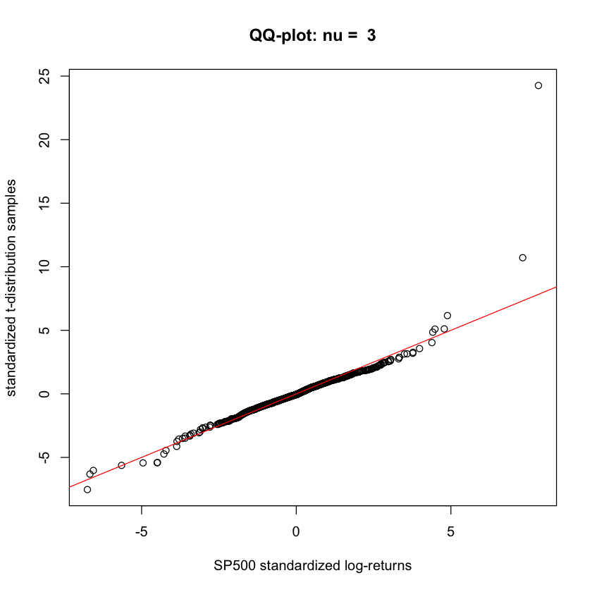
When $\nu = 3$, we can produce QQ-plot with the best fit. When $\nu = 2.1$, both right and left tails are too heavy. Also when $\nu = 4$, left tail is heavy. When $\nu = 3$, we can check the amost every points are on the red line.

(6. b)

(b) In the previous part, we have obtained using graphical methods a rough fit of the SP500 log-returns via the follwing model:

\[r_t = log(S_t) - log(S_{t - 1}) = \mu + \sigma \epsilon_{t} \\\]

where $\epsilon_{t}$ follow the standardized t-distribution with ν degrees of freedom and St is the value of the SP500 index on day t.

Read Problem 4 on page 13 of Ruppert & Matteson. Modify the code therein where the returns are modeled as in (1) and write an R-function that takes as an input the mean $\mu$ and the standard deviation $\sigma$ of the log-returns, the parameter $\nu$ of the degrees of freedom for the standardized t-distribution, and niter. The output of the function should be the simulation-based estimate of the probability of default for the hedge fund.

Produce a table or a graph with the default probabilities as a function of $\nu > 2$ and the volatility $\sigma$. Comment on how do the volatility and the weight of the tail (represented by the parameter $\nu$) affect the default probability. Note: Initially, use $\mu = 0.05 / 253$ and $\sigma = 0.23 / \sqrt{253}$ as in the text and vary $\nu$. Then you can fix a value of $\nu$ and vary $\sigma$. Feel free to also produce heat-map images or 2-way tables of the default probability for a range of values of $\nu$ and $\sigma$.

Solution

default_prob <- function(mu, sd, df, niter){
    below = rep(0, niter)
    set.seed(2023)
    
    for (i in 1:niter){
        e = fGarch::rstd(45, nu = df)
        logPrice = log(1e6) + cumsum(mu + (sd / sqrt(253)) * e)
        minlogP = min(logPrice)
        below[i] = as.numeric(minlogP < log(950000))
    }
    
    return (mean(below))
}

niter = 1e5
mu = 0.05 / 253

df_list = seq(2.1, 3.5, 0.1)
sd_list = seq(0.35, 0.8, 0.05)

results = matrix(0, nrow = length(df_list), ncol = length(sd_list),
                 dimnames = list(df_list, sd_list))

# for (df_idx in 1:length(df_list)){
#     for (sd_idx in 1:length(sd_list)){
#         results[df_idx, sd_idx] = default_prob(mu, sd_list[sd_idx], df_list[df_idx], niter)
#     }
# } -> this code make default_probability.txt file 

require(ggplot2)
require(reshape2)

results = read.table("data/default_probability.txt", header = TRUE, row.names = 1)
results = as.matrix(results)
rownames(results) = df_list
colnames(results) = sd_list

results = round(results, 4)
result_melt = melt(results)

par(mfrow = c(1, 1))
options(repr.plot.width=15, repr.plot.height=8)

ggp = ggplot(data = result_melt, aes(x=Var1, y=Var2, fill= value)) + 
      geom_tile() + 
      geom_text(aes(label = value)) + 
      labs(y = "Volatility", x = "Degree of freedom", title = "Default Probability") +
      scale_x_continuous(breaks = df_list) + 
      scale_y_continuous(breaks = sd_list) + 
      scale_fill_gradient(low="white", high="red")

ggp

png

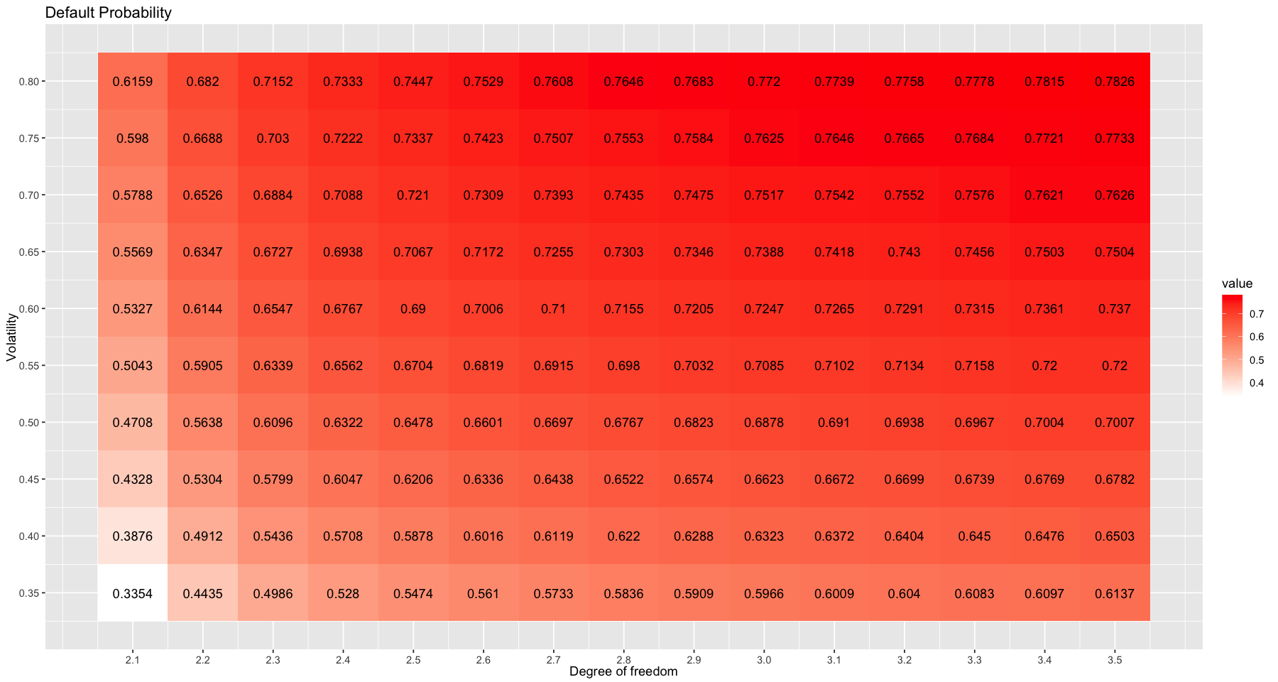
The higher the degree of freedom, the heavier the tail and the higher the default probability.
The higher the volatility, the higher the default probability.

Youngjun Woo

Problem 1

(1. a)

(1. b)

(1. c)

Problem 2

(2. a)

(2. b)

(2. c)

Problem 3

(3. a)

(3. b)

Problem 4

(4. a)

(4. b)

(4. c)

Problem 5

(5. a)

(5. b)

(5. c)

Problem 6

(6. a)

(6. b)