HW2

Topics: Mixture model, Method of moment, Kurtosis, Skewness, KDE(Kernal Density Estimator), MLE(Maximum Likelihood Estimation)

---

Problem 1

Consider the mixture model

\[f(x;p,\mu,\sigma,c\sigma) = p f(x; \mu,\sigma ) + (1-p) f(x; \mu, c \sigma),\]

where $f(x;\mu, \sigma)$ is the probability density of the Normal distribution with zero mean $\mu$ and variance $\sigma^2$.

(1. a)

Let $X \sim f(x;p,\mu,\sigma,c\sigma)$. Compute

\[\mathbb{E} |X - \mu| \ \ \mbox{ and } \ \ \mathbb{E} [(X -\mu)^2]\]

in terms of the parameters $p$, $c$ and $\sigma$.

Solution

We have that

\[\begin{aligned} \mathbb{E}|X - \mu| &= \int_{-\infty}^{\infty}|x - \mu|f(x; p, \mu, \sigma, c\sigma)dx \\ &= p\int_{-\infty}^{\infty}|x - \mu|\frac{1}{\sqrt{2\pi}\sigma}e^{-\frac{(x - \mu) ^ 2}{2\sigma^2}}dx \\ &+ (1 - p)\int_{-\infty}^{\infty}|x - \mu|\frac{1}{\sqrt{2\pi}c\sigma}e^{-\frac{(x - \mu)^2}{2c^2\sigma^2}}dx \\ &= p\int_{-\infty}^{\infty}|y|\frac{1}{\sqrt{2\pi}\sigma}e^{-\frac{y^2}{2\sigma^2}}dy + (1 - p)\int_{-\infty}^{\infty}|y|\frac{1}{\sqrt{2\pi}c\sigma}e^{-\frac{y^2}{2c^2\sigma^2}}dy \\ &= 2p \int_{0}^{\infty}y\frac{1}{\sqrt{2\pi}\sigma}e^{-\frac{y^2}{2\sigma^2}}dy + 2(1 - p)\int_{0}^{\infty}y \frac{1}{\sqrt{2\pi}c\sigma}e^{-\frac{y^2}{2c^2\sigma^2}}dy, \end{aligned}\]

where we have used the change of variables $y = x − \mu$ and the symmetry of the integrands. Working with the first integral in the last expression above,

\[2p\int_{0}^{\infty}y\frac{1}{\sqrt{2\pi}\sigma}e^{-\frac{y^2}{2\sigma^2}}dy = \frac{2p}{\sqrt{2\pi}\sigma}[-\sigma^2e^{-y^2/(2\sigma^2)}]_{0}^{\infty} = \sqrt{\frac{2}{\pi}}\sigma p.\]

Similarly,

\[2(1 - p)\int_{0}^{\infty}y\frac{1}{\sqrt{2\pi}c \sigma}e^{-\frac{y^2}{2c^2\sigma^2}}dy = \sqrt{\frac{2}{\pi}}c\sigma(1 - p)\]

Putting those two together, we have

\[\mathbb{E}|X - \mu| = \sqrt{\frac{2}{\pi}}\sigma(p + (1 - p)c)\]

Now for the second expectation,

\[\begin{aligned} \mathbb{E}(X - \mu)^2 &= \int_{-\infty}^{\infty}(x - \mu)^2 f(x; p, \mu, \sigma, c\sigma)dx \\ &= p \int_{-\infty}^{\infty}(x - \mu)^2 \frac{1}{\sqrt{2 \pi}\sigma}e^{-\frac{(x - \mu)^2}{2\sigma^2}}dx \\ &+ (1 - p)\int_{-\infty}^{\infty}(x - \mu)^2\frac{1}{\sqrt{2\pi}c\sigma}e^{-\frac{(x - \mu)^2}{2c^2\sigma^2}}dx \\ &= pVar(x_1) + (1 - p)Var(X_2) \end{aligned}\]

where $X_1 \sim N(\mu, \sigma^2)$ and $X_2 \sim N(\mu, c^2\sigma^2)$. So,

\[\mathbb{E}(X - \mu)^2 = \sigma^2(p + (1 - p)c ^ 2)\]

(1. b)

The parameter $\sigma>0$ is known. Given an iid sample $X_1,\dots,X_n \sim f(x;p,\mu,\sigma,c\sigma)$, construct estimators for the unknown parameters $p,\ \mu$, $c>0$ using the (generalized) method of moments.

Hint: You can estimate $\mu$ via $\overline X_n$. Consider the statistics

\[\hat m_1 := \frac{1}{n} \sum_{i=1}^n |X_i-\overline X_n|\ \ \mbox{ and } \ \ \hat m_2 := \frac{1}{n} \sum_{i=1}^n (X_i-\overline X_n)^2,\]

which estimate $\mathbb{E} |X - \mu|$ and $\mathbb{E} [(X - \mu)^2]$, respectively. Using the formulae derived in (1.a), solve for $p$ and $c$.

Solution

We need to solve the following equations for $\hat{\mu}, \hat{p}, \hat{c}$:

\[\begin{aligned} &\bar{X_n} = \hat{\mu} \\ &\hat{m_1} = \sqrt{\frac{2}{\pi}}\sigma(\hat{p} + (1 - \hat{p})\hat{c}) \\ &\hat{m_2} = \sigma^2(\hat{p} + (1 - \hat{p})\hat{c}^2) \end{aligned}\]

After trivial algebra, we obtain

\[\begin{aligned} &\hat{\mu} = \bar{X_n} \\ &\hat{p} = \frac{\hat{m_2} - \frac{\pi}{2}\hat{m_1}^2}{\hat{m_2} - 2\sigma\hat{m_1}\sqrt{\frac{\pi}{2}} + \sigma^2} \\ &\hat{c} = \frac{\frac{\hat{m_1}\sqrt{\pi / 2}}{\sigma} - \hat{p}}{1 - \hat{p}} \end{aligned}\]

(1. c)

Let $\mu=0.1$, $p=0.3$, $\sigma=1$ and $c=1.3$. Simulate $n=500$ independent samples from the above mixture model and compute the point estimators from part (1.b). Repeat this simulation $N=1000$ times and produce a table with the empirical $95\%$ confidence intervals for $\mu$, $p$ and $c$.

Solution

n = 500
iter = 1000
mu = 0.1
sig = 1
p = 0.3
c = 1.3

m = c()
phat = c()
chat = c()

for  (i in c(1:iter)){
  U = runif(n)
  Z = rnorm(n)
  
  X = (mu + Z * sig) * (U < p) +
      (mu + Z * c * sig) * (U >= p)
  xbar = mean(X)
  m1 = 1/n * sum(abs(X - xbar))
  m2 = 1/n * sum((X - xbar)**2)
  p_est = (m2 - pi * m1**2 / 2) / (m2 - 2 * sig * m1 * sqrt(pi/2) + sig**2)
  c_est = (m1 * sqrt(pi/2) / sig - p_est) / (1 - p_est)
  m = c(m, xbar)
  phat = c(phat, p_est)
  chat = c(chat, c_est)
}

m_quantile = quantile(m, probs = c(0.025, 0.975))
p_quantile = quantile(phat, probs = c(0.025, 0.975))
c_quantile = quantile(chat, probs = c(0.025, 0.975))
res = matrix(c(m_quantile, p_quantile, c_quantile), nrow = 3, ncol = 2, byrow = T)
dimnames(res) = list(c("mu", "p", "c"), 
                     c("2.5 percentile", "97.5 percentile"))
res

A matrix: 3 × 2 of type dbl

	2.5 percentile	97.5 percentile
mu	-0.01073616	0.2111208
p	-5.05635001	2.5861865
c	0.97928999	1.6488707

Problem 2

Consider the $t$-distributed random variable $T = Z/\sqrt{Y/\nu}$, where $Z \sim{\mathcal N}(0,1)$ and $Y\sim {\rm Gamma}(\nu/2,1/2),\ \nu>0$ be two independent random variables.

(2. a)

Assuming that $\nu>4$, compute the kurtosis of $T$, that is

\[{\rm kurt}(T) = \mathbb{E} \left( \frac{(T-\mu)^4}{\sigma^4} \right),\]

in terms of $\nu$, where $\mu = \mathbb{E}(T)$ and $\sigma^2 = {\rm Var}(T)$.

Solution

\(\begin{aligned} {\rm kurt}(T) &= \mathbb{E} \left( \frac{(T-\mu)^4}{\sigma^4} \right) \\ &= \mathbb{E} \left( \frac{T^4 -\mu \cdot T^3 + \mu^2 \cdot T^2 - \mu^3 \cdot T + \mu ^ 4}{\sigma^4} \right) \\ &= \frac{1}{\sigma ^ 4} \cdot \mathbb{E} \left( T ^ 4 \right) - \frac{\mu}{\sigma ^ 4} \cdot \mathbb{E} \left( T ^ 3 \right) + \frac{\mu ^ 2}{\sigma ^ 4} \cdot \mathbb{E} \left( T ^ 2 \right) - \frac{\mu ^ 3}{\sigma ^ 4} \cdot \mathbb{E} \left( T \right) + \frac{\mu ^ 4}{\sigma ^ 4} \\ \end{aligned}\) Since $\mu = \mathbb{E} \left( T \right) = 0$, and $\sigma ^ 2 = {\rm Var}(T) = \frac{\nu}{\nu - 2}$, \
${\rm kurt}(T) = \frac{(\nu - 2) ^ 2}{\nu ^ 2} \cdot \mathbb{E} \left(T ^ 4 \right)$ \
Note that $\mathbb{E} \left(T ^ 4 \right) = \mathbb{E} \left(\frac{Z ^ 4}{Y ^ 2 / \nu ^ 2}\right) = \nu ^ 2 \cdot \mathbb{E} \left(Z ^ 4\right) \cdot \mathbb{E} \left(Y ^ {-2}\right)$

Here, $\mathbb{E} \left(Y ^ k\right) = (\frac{1}{2}) ^ {-k} \cdot \frac{\Gamma(\frac{\nu}{2} + k)}{\Gamma(\frac{\nu}{2})}$ for $k > -\frac{\nu}{2}$

So,

\[\begin{aligned} \mathbb{E} \left(Y ^ {-2}\right) &= (\frac{1}{2}) ^ {2} \cdot \frac{\Gamma(\frac{\nu}{2} - 2)}{\Gamma(\frac{\nu}{2})} \\ &= \frac{1}{(\nu - 2)(\nu - 4)} \end{aligned}\]

Also, since Z follows standard normal distribution, skewness = $\mathbb{E} \left( Z ^ 3\right) = 0$ and kurtosis = $\mathbb{E} \left( Z ^ 4\right) = 3$.

\[\begin{aligned} \therefore \mathbb{E} \left(T^4\right) &= \nu ^ 2 \cdot \mathbb{E} \left(Z ^ 4\right) \cdot \mathbb{E} \left(Y ^ {-2}\right) &= \frac{3 \cdot \nu ^ 2}{(\nu - 2)(\nu - 4)} \end{aligned}\] \[\begin{aligned} \rightarrow {\rm kurt}(T) &= \frac{(\nu - 2) ^ 2}{\nu ^ 2} \cdot \mathbb{E} \left(T ^ 4\right) \\ &= \frac{(\nu - 2) ^ 2}{\nu ^ 2} \cdot \frac{3 \cdot \nu ^ 2}{(\nu - 2)(\nu - 4)} \\ & = \frac{3 \cdot (\nu - 2)}{\nu - 4} \end{aligned}\]

(2. b)

Suppose that $T_1,\dots,T_n$ are independent realizations form the above $t$-distribution model. Estimate $\nu$ if the sample kurtosis

\[\frac{1}{n} \sum_{i=1}^n \left(\frac{ T_i -\overline T_n}{s_n} \right)^4 = 9,\]

where $s_n^2 = n^{-1} \sum_{i=1}^n (T_i - \overline T_n)^2$.

Solution

\[\begin{aligned} & \mathbb{E} \left( \frac{(T-\mu)^4}{\sigma^4} \right) = \frac{1}{n}\sum_{i = 1}^{n}{(\frac{T_i - \overline T_n}{S_n}) ^ 4} \\ & \rightarrow \frac{3 \cdot (\nu - 2)}{\nu - 4} = 9 \\ & \rightarrow \nu = 5 \\ & \therefore \hat {\nu} = 5 \\ \end{aligned}\]

Problem 3

Let $p_1 = 0.2, p_2 = 0.5$ and $p_3 = 0.3$, consider the mixture density

\[f(x) = p_1 f_1(x) + p_2 f_2(x) + p_3 f_3(x),\]

where $f_i$ are ${\mathcal N}(\mu_i,\sigma_i^2),\ i=1,2,3$ densities.

(3. a)

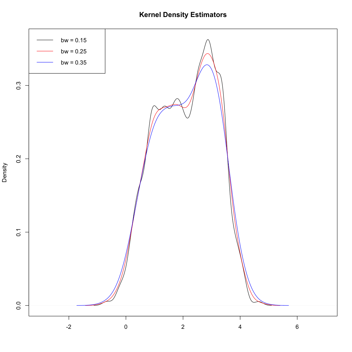
Set $\mu_i = i,\ i=1,2,3$, $\sigma_2 =1$ and $\sigma_1=\sigma_3=0.5$. Simulate $n=500$ points from this mixture distribution and estimate the density $f(x)$ using a kernel density estimator with bandwidth $h$, for three values of $h$. Plot on the same graph the resulting KDEs.

Solution

options(repr.plot.width=10, repr.plot.height=10)

p1 = 0.2
p2 = 0.5
p3 = 0.3

mu1 = 1
mu2 = 2
mu3 = 3

sig1 = 0.5
sig2 = 1
sig3 = 0.5

n = 500

U = runif(n)
Z = rnorm(n)

X = (mu1 + sig1 * Z) * (U < p1) + 
    (mu2 + sig2 * Z) * (U >= p1) * (U < p1 + p2) +
    (mu3 + sig3 * Z) * (U >= p1 + p2)

d1 = density(X, bw = 0.15)
d2 = density(X, bw = 0.25)
d3 = density(X, bw = 0.35)

plot(d1, xlab = "",ylab = "Density",
     main = "Kernel Density Estimators", xlim = c(-5+2,5+2))
lines(d2, col = "red")
lines(d3, col = "blue")
legend("topleft", legend = c("bw = 0.15","bw = 0.25","bw = 0.35"),
col = c("black", "red", "blue"), lwd = c(1,1))

(3. b)

Knowing the true density $f$, write an R-function that takes as inputs the simulated data and the bandwidth $h$ and computes exaclty the quantity \(ISE(h) := \int_{\mathbb{R}} (\hat f_h(x) - f(x))^2 dx.\)

Solution

Recall that for the Gaussian kernel, we have that

\[\hat{f_h}(x) = \frac{1}{nh\sqrt{2\pi}}\sum_{i = 1}^{n}e^{-\frac{(x - X_i)^2}{2h^2}}.\]

We have that

\[\begin{aligned} ISE(h) &= \int_{\mathbb{R}}(\hat{f_h}(x) - f(x))^2dx \\ &= \int_{\mathbb{R}}\hat{f_h}^2(x)dx - 2\int_{\mathbb{R}}\hat{f_h}(x)f(x)dx + \int_{\mathbb{R}}f^2(x)dx \end{aligned}\]

We will start with the first term. We have,

\[\begin{aligned} \int_{\mathbb{R}}\hat{f_h}^2(x)dx &= \frac{1}{2\pi n^2 h^2}\int_{\mathbb{R}}(\sum_{i = 1}^{n}e^{-\frac{(x - X_i)^2}{2h^2}})^2dx \\ &= \frac{1}{2\pi n^2 h^2}\int_{\mathbb{R}}(\sum_{i_1, i_2 = 1}^{n}e^{-\frac{(x - X_{i_1})^2 + (x - X_{i_2})^2}{2h^2}})^2dx \\ &= \sum_{i_1, i_2 = 1}^{n}\frac{1}{2\pi n^2 h^2}\int_{\mathbb{R}}e^{-\frac{2x^2 - 2x(X_{i_1} + X_{i_2}) + X_{i_1}^2 + X_{i_2}^2}{2h^2}})^2dx \\ &= \sum_{i_1, i_2 = 1}^{n}\frac{1}{2\pi n^2 h^2}\int_{\mathbb{R}}e^{-\frac{2(x^2 - 2x\frac{X_{i_1} + X_{i_2}}{2} + (\frac{X_{i_1} + X_{i_2}}{2})^2)}{2h^2}})^2dx\cdot e^{- \frac{X_{i_1}^2 + X_{i_2}^2 - 2(\frac{X_{i_1} + X_{i_2}}{2})^2}{2h^2}} \\ &= \sum_{i_1, i_2 = 1}^{n}\frac{1}{2\pi n^2 h^2}\sqrt{2\pi}\frac{h}{\sqrt{2}}e^{-\frac{(X_{i_1} - X_{i_2})^2}{4h^2}} \\ &= \sum_{i_1, i_2 = 1}^{n} \frac{1}{2n^2 h \sqrt{\pi}}e^{-\frac{(X_{i_1} - X_{i_2})^2}{4h^2}} \end{aligned}\]

Similarly, we obtain

\[- 2\int_{\mathbb{R}}\hat{f_h}(x)f(x)dx = -2\sum_{i = 1}^{n}\sum_{j = 1}^{3}\frac{p_j}{n\sqrt{2\pi}\sqrt{h^2 + \sigma_j^2}}e^{-\frac{(X_i - \mu)^2}{2(\sigma_j^2 + h^2)}}\\ \int_{\mathbb{R}}f^2(x)dx = \sum_{j_1, j_2 = 1}^{3}\frac{p_{j_1}p_{j_2}}{\sqrt{2\pi}\sqrt{\sigma_{j_1}^2 + \sigma_{j_2}^2}}e^{-\frac{(\mu_{j_1} - \mu_{j_2})^2}{2(\sigma_{j_1}^2 + \sigma_{j_2}^2)}}\]

p = c(p1, p2, p3)
mu = c(mu1, mu2, mu3)
sig = c(sig1, sig2, sig3)

ISE <-function(h, data = X){
    n = length(X)
    A = B = C = 0;
    for (i1 in 1:n){
        for (i2 in 1:n){
            A = A + 1/(2* n**2 * h * sqrt(pi)) *
            exp(-(X[i1]-X[i2])**2 / (4 * h**2))
        }
    }

    for (i in 1:n){
        for (j in 1:3){
            B = B - 2 * p[j] / (n * sqrt(2 * pi) * sqrt(h**2 + sig[j]**2))*
            exp(-(X[i] - mu[j])**2 / (2 * (sig[j]**2 + h**2)))
        }
    }
    
    for (j1 in 1:3){
        for (j2 in 1:3){
            C = C + p[j1] * p[j2] / (sqrt(2 * pi) * sqrt(sig[j1]**2 + sig[j2]**2)) *
            exp(-(mu[j1] - mu[j2])**2 / (2 * (sig[j1]**2 + sig[j2]**2)))
        }
    }

    return(A+B+C)
}

(3. c)

Plot the quantity $ISE(h)$ as a function of $h$ and determine visually the best value of $h= h^$. Plot the resulting KDE $\hat f_{h^}(x)$ as a function of $x$.

Solution

options(repr.plot.width=12, repr.plot.height=10)

ISE_list = c()

h_val= (15:35)/100

for (h in h_val){
    ISE_list = c(ISE_list, ISE(h))
}

par(mfrow=c(1,2))

plot(h_val, ISE_list, type = "l", xlab = "h", ylab = "ISE(h)")
h_star = h_val[which.min(ISE_list)]
abline(v = h_star, col = "blue")
abline(h = min(ISE_list), col = "red")
d = density(X, bw = h_star, kernel = "gaussian")
plot(d$x, d$y, type = "l", col = "red", ylim = c(0,0.5), xlab = "x",
     ylab = "density")
lines(d$x, (p1 * dnorm(d$x, mean = mu1, sd = sig1) +
            p2 * dnorm(d$x, mean = mu2, sd = sig2) +
            p3 * dnorm(d$x, mean = mu3, sd = sig3)))
legend("topleft", legend = c("KDE for hstar","Actual density"),
       col = c("red","black"), lwd = c(1,1))

Problem 4

Load the data set sp500_full.csv found in the data folder on Canvas.

(4. a)

Using maximum likelihood, fit the skewed t-distribution discussed in class to the daily returns (variable sprtrn) of the sp500 time series. Namely, consider the range of years 1962, 1963, …, 2021. For the samples of daily returns corresponding to each year $y$ in this range, obtain $\hat \theta_{MLE}(y),\ y=1962,\ldots,2021$. Do so by using the optim function in R in two differnt ways (1) using the method “BFGS” and (2) via “Nelder-Mead”. Compare the results and comment on the stability of each of the optimization methods.

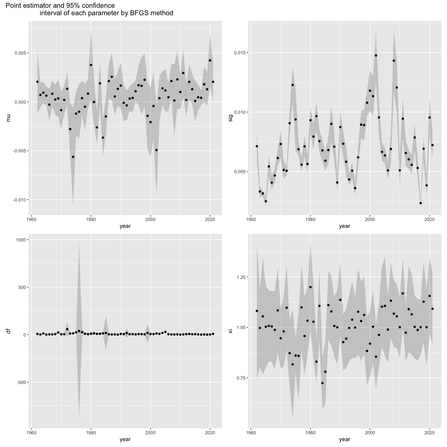
Finally, using the Hessian estimate from the optimization routine, for each of the 4 parameters $\mu,\sigma,\nu,$ and $\xi$, produce a plot of the point estimate along with point-wise 95\% confidence intervals as a function of time (years).

Solution

require("ggplot2")
require("patchwork")

sp= read.csv("data/sp500_full.csv")
sp_t <- as.Date(as.character((sp$caldt)), format = "%Y%m%d")
idx = which((sp_t >= "1962-01-01") & (sp_t <= "2021-12-31"))
sp_t = sp_t[idx]
sp_rtrn = sp$sprtrn[idx]

skew_t_dist = function(x, xi, df) {
  (dt(x * xi ^ (sign(x)), df = df) * 2 * xi / (1 + xi ^ 2))
}

nlog_lik_skew_t = function(theta) {
  -sum(log(skew_t_dist((x - theta[1]) / theta[2],
                       df = theta[3], xi = theta[4])) - log(theta[2]))
}

y_list = seq(1962, 2021)
results_bfgs = c()
results_nm = c()

for (y in y_list) {
  options(warn=0)
  target_y_idx = (format(sp_t, format = "%Y") == format(y, format = "%Y"))
  x = sp_rtrn[target_y_idx & !is.na(sp_rtrn)]

  start = c(mean(x), sd(x) + 0.05, 0.1, 1)

  fit_st_bfgs = optim(start, nlog_lik_skew_t, hessian = T,
                      method = "L-BFGS-B", lower = c(-1, 0.001, 1, 0.001))

  fit_st_lm = optim(start, nlog_lik_skew_t, hessian = T,
                    method = "Nelder-Mead")

  cov = solve(fit_st_lm$hessian)
  se = sqrt(diag(cov))

  results_bfgs = rbind(results_bfgs,
                       c(y, fit_st_bfgs$par, fit_st_bfgs$par - 1.96 * se,
                        fit_st_bfgs$par + 1.96 * se))
  results_nm = rbind(results_nm,
                     c(y, fit_st_lm$par, fit_st_lm$par - 1.96 * se,
                      fit_st_lm$par + 1.96 * se))
}

col_names = c("year", "mu", "sig", "df", "xi",
              "mu_lb", "sig_lb", "df_lb", "xi_lb",
              "mu_ub", "sig_ub", "df_ub", "xi_ub")

colnames(results_bfgs) = col_names
results_bfgs = data.frame(results_bfgs)

colnames(results_nm) = col_names
results_nm = data.frame(results_nm)


rs_etm = rbind(cbind(results_bfgs[, "mu"], "mu", "BFGS"),
               cbind(results_bfgs[, "sig"], "sig", "BFGS"),
               cbind(results_bfgs[, "df"], "df", "BFGS"),
               cbind(results_bfgs[, "xi"], "xi", "BFGS"),

               cbind(results_nm[, "mu"], "mu", "NM"),
               cbind(results_nm[, "sig"], "sig", "NM"),
               cbind(results_nm[, "df"], "df", "NM"),
               cbind(results_nm[, "xi"], "xi", "NM"))

colnames(rs_etm) = c("value", "parameter", "method")
rs_etm = data.frame(rs_etm)
rs_etm$value = as.numeric(rs_etm$value)

options(repr.plot.width=12, repr.plot.height=12)

p1 = ggplot(rs_etm[rs_etm$parameter == "mu", ],
            aes(x = parameter, y = value, color = method)) +
        geom_boxplot(outlier.shape = NA) +
        coord_cartesian(
          ylim = quantile(rs_etm[rs_etm$parameter == "mu", ]$value, c(0.1, 0.9))
        ) +
        theme(axis.text.x = element_blank(),
              axis.ticks.x = element_blank()) +
        labs(x = "Mu")

p2 = ggplot(rs_etm[rs_etm$parameter == "sig", ],
            aes(x = parameter, y = value, color = method)) +
        geom_boxplot(outlier.shape = NA) +
        coord_cartesian(
          ylim = quantile(rs_etm[rs_etm$parameter == "sig", ]$value, c(0.1, 0.9))
        ) +
        theme(axis.text.x = element_blank(),
              axis.ticks.x = element_blank()) +
        labs(x = "Sigma")

p3 = ggplot(rs_etm[rs_etm$parameter == "df", ],
            aes(x = parameter, y = value, color = method)) +
        geom_boxplot(outlier.shape = NA) +
        coord_cartesian(
          ylim = quantile(rs_etm[rs_etm$parameter == "df", ]$value, c(0.1, 0.9))
        ) +
        theme(axis.text.x = element_blank(),
              axis.ticks.x = element_blank()) +
        labs(x = "Df")

p4 = ggplot(rs_etm[rs_etm$parameter == "xi", ],
            aes(x = parameter, y = value, color = method)) +
        geom_boxplot(outlier.shape = NA) +
        coord_cartesian(
          ylim = quantile(rs_etm[rs_etm$parameter == "xi", ]$value, c(0.1, 0.9))
        ) +
        theme(axis.text.x = element_blank(),
              axis.ticks.x = element_blank()) +
        labs(x = "Xi")

p1 + p2 + p3 + p4 +
  plot_annotation("Compare the stability of estimated
                  parameters between BFGS and N-M methods")

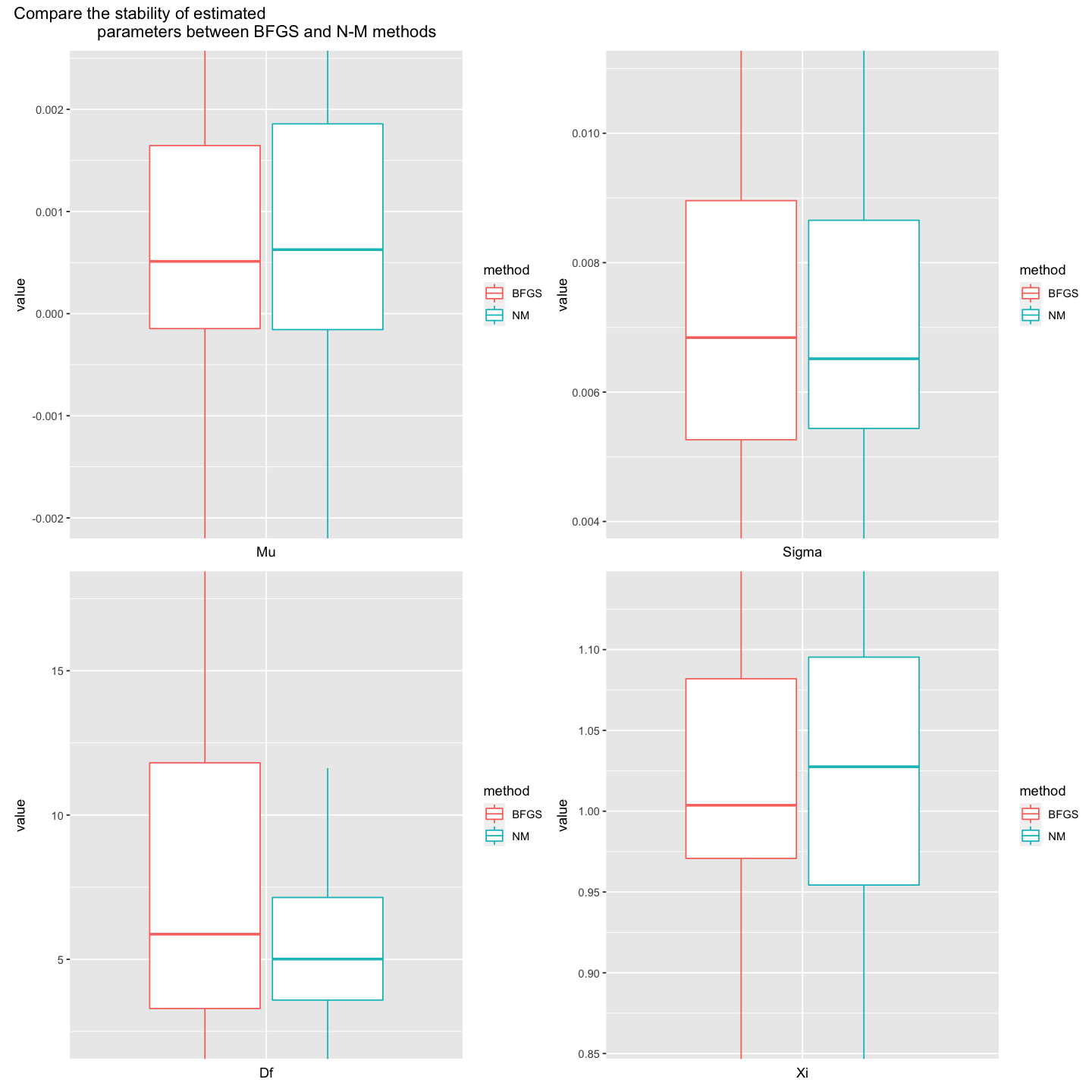
• Both method shows similar estimation result on mu, sigma, and xi parameters. In the above box plots of mu, sigma, and xi, we can see the similar quantile values of estimated parameters from both methods. However, in the case of df, we can check the less stability of estimation from BFGS method than N-M method. In BFGS method, estimated values of df from BFGS method shows broader range compared to those from N-M method.

p1 = ggplot(results_bfgs, aes(x = year, y = mu)) +
  geom_point() +
  geom_ribbon(aes(ymin = mu_lb, ymax = mu_ub), alpha = 0.2)

p2 = ggplot(results_bfgs, aes(x = year, y = sig)) +
  geom_point() +
  geom_ribbon(aes(ymin = sig_lb, ymax = sig_ub), alpha = 0.2)

p3 = ggplot(results_bfgs, aes(x = year, y = df)) +
  geom_point() +
  geom_ribbon(aes(ymin = df_lb, ymax = df_ub), alpha = 0.2)

p4 = ggplot(results_bfgs, aes(x = year, y = xi)) +
  geom_point() +
  geom_ribbon(aes(ymin = xi_lb, ymax = xi_ub), alpha = 0.2)

p1 + p2 + p3 + p4 +
  plot_annotation("Point estimator and 95% confidence
                  interval of each parameter by BFGS method")

p1 = ggplot(results_nm, aes(x = year, y = mu)) +
  geom_point() +
  geom_ribbon(aes(ymin = mu_lb, ymax = mu_ub), alpha = 0.2)

p2 = ggplot(results_nm, aes(x = year, y = sig)) +
  geom_point() +
  geom_ribbon(aes(ymin = sig_lb, ymax = sig_ub), alpha = 0.2)

p3 = ggplot(results_nm, aes(x = year, y = df)) +
  geom_point() +
  geom_ribbon(aes(ymin = df_lb, ymax = df_ub), alpha = 0.2)

p4 = ggplot(results_nm, aes(x = year, y = xi)) +
  geom_point() +
  geom_ribbon(aes(ymin = xi_lb, ymax = xi_ub), alpha = 0.2)

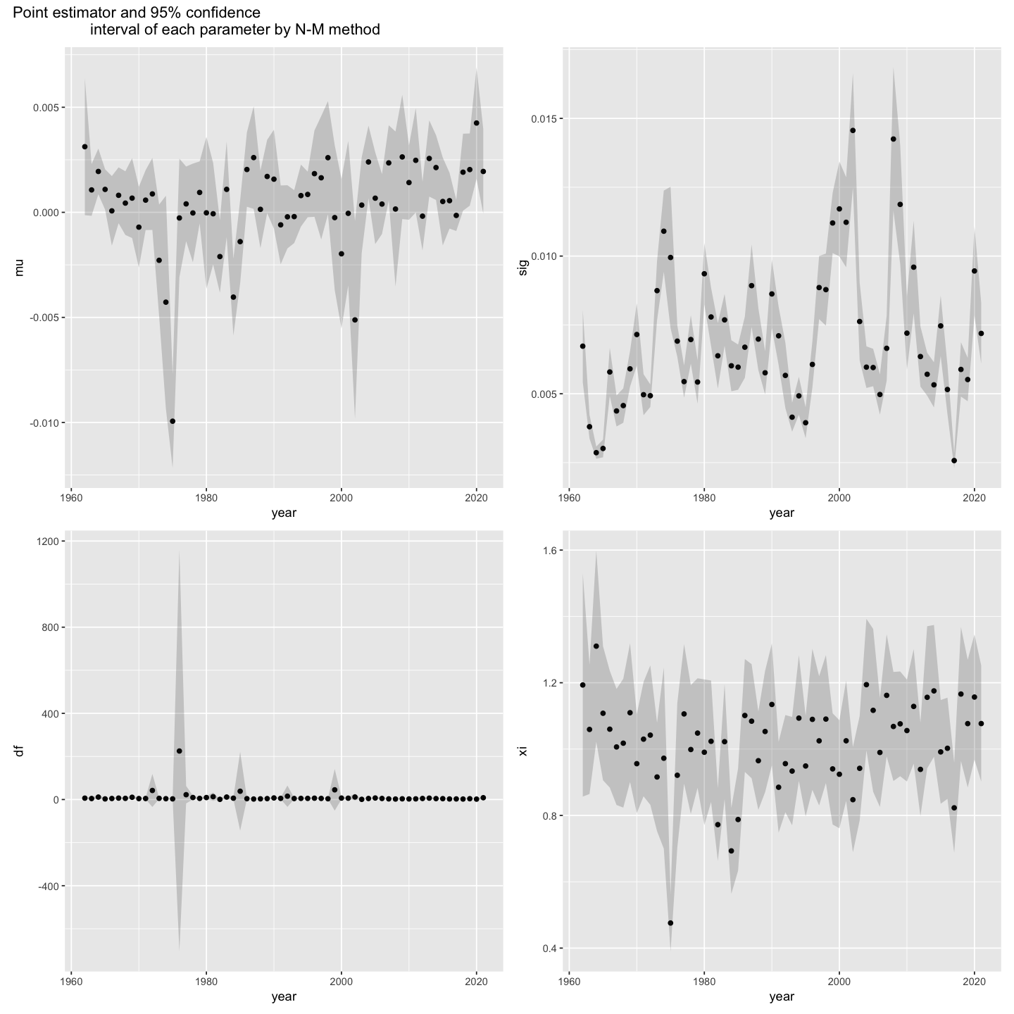
p1 + p2 + p3 + p4 +
  plot_annotation("Point estimator and 95% confidence
                  interval of each parameter by N-M method")

(4. b)

Consider the plot the estimated degrees of freedom parameter $\hat \nu(y)$ as a function of time $y$ (in years) from part (a). Which years $y$ seem to have relatively heavy-tailed returns? Are there any years for which the estimated model has infinite variance? Explain and plot the time series of the daily returns for one of these years.

Solution

• If we check the above point estimator and CI plot, estimated df under N-M method shows a very wide range of CI in 1976 year. So 1976 seems to have relatively heavy-tailed returns. If we check the variance of that year, the variance is 225308. This variance is the biggest value among all years of N-M method. Below plot shows thhe daily returns for the 1976 year.

(4. c)

Consider the confidence intervals for the skewness parameter estimates obtained in part (a). Identify during which years (if any) the skewness paramter $\xi$ is likley to be significantly different from $1$. Ignoring multiple testing issues, test the corresponding (two-sided) hypothesis at a level of 5\%.

Plot the kernel density estimator for the daily returns for one of these “skewed” years and on the same plot display (in different line-style/color) the density of the estimated skewed t-model.

Solution

p4 = ggplot(results_nm, aes(x = year, y = xi)) +
geom_point() +
geom_ribbon(aes(ymin = xi_lb, ymax = xi_ub), alpha = 0.2)
p4 + plot_annotation("Point estimator and 95% confidence
interval of xi parameter by N-M method")

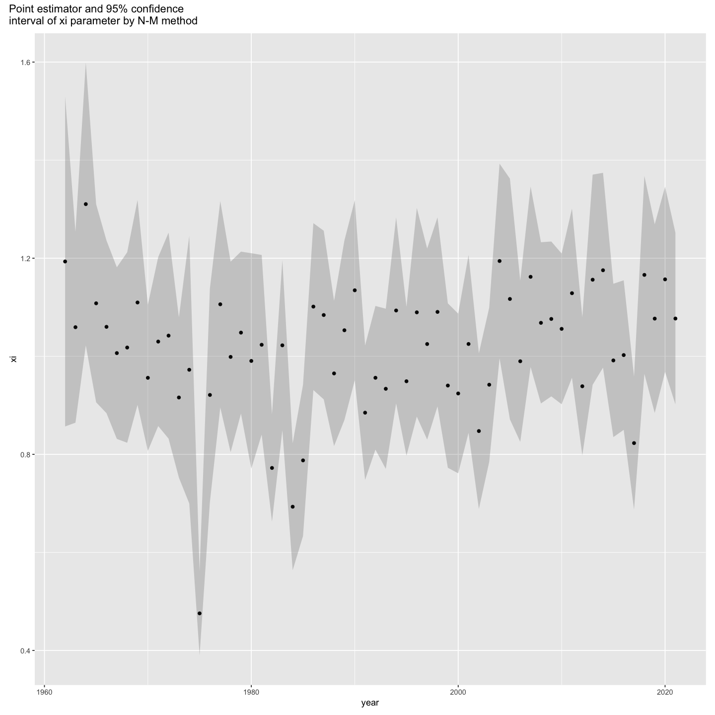
• In the above plot, the skewness parameter is likely to be significantly different from 1 during 1975. Let’s check the confidence interval of xi in 1975 for hypothesis test.

results_nm[results_nm$xi == min(results_nm$xi),
c("year", "xi", "xi_lb", "xi_ub")]

A data.frame: 1 × 4

	year	xi	xi_lb	xi_ub
	<dbl>	<dbl>	<dbl>	<dbl>
14	1975	0.4756608	0.3899451	0.5613764

• If we set H0: xi = 1, H1: otherwise, then since 95\% confidence interval doesn’t contain 1, there is a statistically significant evidence to reject H0.

x  = sp_rtrn[(format(sp_t, format = "%Y") == format(1975, format = "%Y"))]
x = sort(x)
X_density = density(x)

theta = results_nm[results_nm$year == "1975", c("mu", "sig", "df", "xi")]
theta

h = 1.06 * theta$sig * length(x) ^ (-1 / 5)

par(mfrow = c(1, 1))

plot(X_density$x, X_density$y, type = "l",
     xlab = "Daily returns", ylab = "Density",
     main = "Compare KDE and Estimated skewed t-model for 1975")
lines(x, skew_t_dist((x - theta$mu) / theta$sig,
                     df = theta$df, xi = theta$xi) * (1 / theta$sig),
      col = "red")
legend("topright", c("KDE", "Estimated skewed t-model"),
       col = c("black", "red"), lwd = 2)

A data.frame: 1 × 4

	mu	sig	df	xi
	<dbl>	<dbl>	<dbl>	<dbl>
14	-0.009940165	0.009949183	3.069062	0.4756608

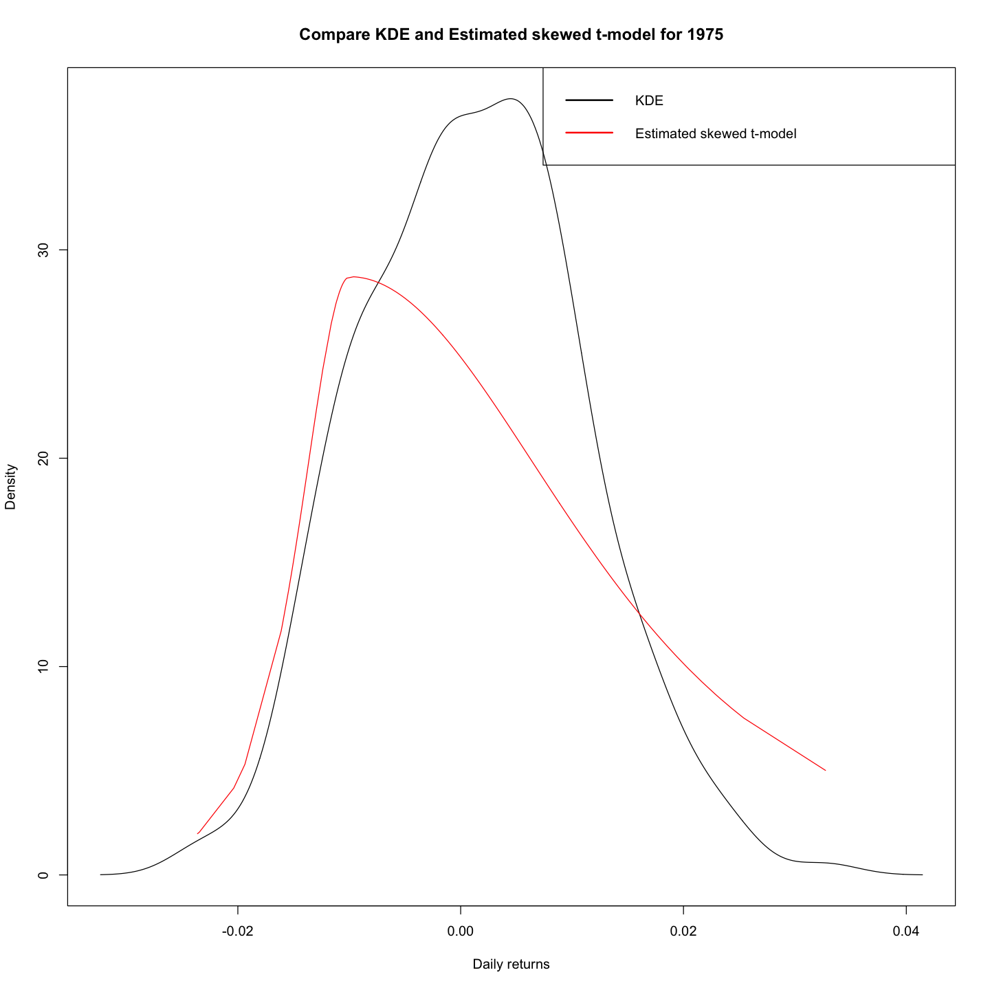
• Above plot shows the KDE for the daily returns for 1975 (skewed years) and the density of the estimated skewed t-model.