3 - 1) Train machine learning models to predict match results (In progress)

import pandas as pd 
import numpy as np 

import matplotlib.pyplot as plt 
import matplotlib.patches as mpatches
import seaborn as sns 
import missingno as msno 

from sklearn.model_selection import train_test_split
from sklearn.pipeline import Pipeline
from sklearn.preprocessing import StandardScaler, OneHotEncoder
from sklearn.model_selection import cross_validate
from sklearn.model_selection import train_test_split
from sklearn import preprocessing

from sklearn.neighbors import KNeighborsClassifier
from sklearn.discriminant_analysis import LinearDiscriminantAnalysis, QuadraticDiscriminantAnalysis 
from sklearn.naive_bayes import GaussianNB
from sklearn.linear_model import LogisticRegression
from sklearn.tree import DecisionTreeClassifier
from sklearn.ensemble import RandomForestClassifier, AdaBoostClassifier
from sklearn import tree
from sklearn.svm import SVC
from sklearn.ensemble import GradientBoostingClassifier
import xgboost as xgb
import lightgbm as lgb

import optuna
from optuna.integration import LightGBMPruningCallback
from optuna.integration import XGBoostPruningCallback
from sklearn.model_selection import GridSearchCV
from sklearn.model_selection import KFold
from sklearn.model_selection import StratifiedKFold

from sklearn.metrics import confusion_matrix
from sklearn.metrics import ConfusionMatrixDisplay
from sklearn.metrics import balanced_accuracy_score
from sklearn.metrics import roc_auc_score
from sklearn.metrics import log_loss
from sklearn.metrics import classification_report

from sklearn.inspection import permutation_importance

import imblearn
from imblearn.over_sampling import SMOTE

import warnings
warnings.filterwarnings('ignore')

pd.set_option('display.max_columns', None)

• We have 5 kinds of variable sets
  • variable set 1: player attributes PC features
  • Variable set 2: betting information features
  • variable set 3: team attributes features
  • variable set 4: goal and win percentage rolling features
  • variable set 5: each team’s Elo rating

df_match_basic = pd.read_csv("../data/df_match_basic.csv")

df_match_player_attr_pcs = pd.read_csv("../data/df_match_player_attr_pcs.csv")

df_match_betting_stat = pd.read_csv("../data/df_match_betting_stat.csv")

df_match_team_num_attr = pd.read_csv("../data/df_match_team_num_attr.csv")

df_team_win_goal_rolling_features = pd.read_csv("../data/df_team_win_goal_rolling_features.csv")

df_match_elo = pd.read_csv("../data/df_match_elo.csv")

• First, let’s predict the match result and compare the result by using each variable sets.

1. Train test split

• Set last season as test set, other seasons as train set.

target_bool = (df_match_basic.match_api_id.isin(df_match_player_attr_pcs.match_api_id)) & \
              (df_match_basic.match_api_id.isin(df_match_betting_stat.match_api_id)) & \
              (df_match_basic.match_api_id.isin(df_match_team_num_attr.match_api_id)) & \
              (df_match_basic.match_api_id.isin(df_team_win_goal_rolling_features.match_api_id)) & \
              (df_match_basic.match_api_id.isin(df_match_elo.match_api_id))
    

target_matches = df_match_basic[target_bool]

test_match_api_id = target_matches[target_matches.season == "2015/2016"].match_api_id
train_match_api_id = target_matches[target_matches.season != "2015/2016"].match_api_id

print(len(train_match_api_id), len(test_match_api_id))

16988 2621

• There are 16,988 train set and 2,621 test set.

2. Baseline accuracy

df_match_basic[df_match_basic.match_api_id.isin(train_match_api_id)].match_result.value_counts()

home_win    7840
away_win    4855
draw        4293
Name: match_result, dtype: int64

sns.countplot(x = df_match_basic[df_match_basic.match_api_id.isin(train_match_api_id)].match_result)

<AxesSubplot:xlabel='match_result', ylabel='count'>

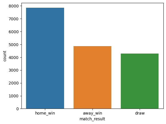
• About 46% of all 16,988 matches were won by the home team.

• That is, if we predict all matches as home team win, then we can achieve about 46% accuracy, that can be used as our baseline accuracy.

• Let’s check the baseline accuracy in the test data set.

df_match_basic[df_match_basic.match_api_id.isin(test_match_api_id)].match_result.value_counts()

home_win    1161
away_win     801
draw         659
Name: match_result, dtype: int64

sns.countplot(x = df_match_basic[df_match_basic.match_api_id.isin(test_match_api_id)].match_result)

<AxesSubplot:xlabel='match_result', ylabel='count'>

• Baseline accuracy in the test dataset is about 44% (1,161 / 2,621)

3. Modeling with all variable sets

3.1. Variable set 1: Player attributes PC features

df_match_player_attr_pcs = df_match_player_attr_pcs.merge(df_match_basic[["match_api_id", "match_result"]], how = "left", on = "match_api_id")

df_match_player_attr_pcs = df_match_player_attr_pcs.set_index("match_api_id")
df_match_player_attr_pcs

	home_player_1_pc_1	home_player_1_pc_2	home_player_1_pc_3	home_player_1_pc_4	home_player_1_pc_5	home_player_2_pc_1	home_player_2_pc_2	home_player_2_pc_3	home_player_2_pc_4	home_player_2_pc_5	home_player_3_pc_1	home_player_3_pc_2	home_player_3_pc_3	home_player_3_pc_4	home_player_3_pc_5	home_player_4_pc_1	home_player_4_pc_2	home_player_4_pc_3	home_player_4_pc_4	home_player_4_pc_5	home_player_5_pc_1	home_player_5_pc_2	home_player_5_pc_3	home_player_5_pc_4	home_player_5_pc_5	home_player_6_pc_1	home_player_6_pc_2	home_player_6_pc_3	home_player_6_pc_4	home_player_6_pc_5	home_player_7_pc_1	home_player_7_pc_2	home_player_7_pc_3	home_player_7_pc_4	home_player_7_pc_5	home_player_8_pc_1	home_player_8_pc_2	home_player_8_pc_3	home_player_8_pc_4	home_player_8_pc_5	home_player_9_pc_1	home_player_9_pc_2	home_player_9_pc_3	home_player_9_pc_4	home_player_9_pc_5	home_player_10_pc_1	home_player_10_pc_2	home_player_10_pc_3	home_player_10_pc_4	home_player_10_pc_5	home_player_11_pc_1	home_player_11_pc_2	home_player_11_pc_3	home_player_11_pc_4	home_player_11_pc_5	away_player_1_pc_1	away_player_1_pc_2	away_player_1_pc_3	away_player_1_pc_4	away_player_1_pc_5	away_player_2_pc_1	away_player_2_pc_2	away_player_2_pc_3	away_player_2_pc_4	away_player_2_pc_5	away_player_3_pc_1	away_player_3_pc_2	away_player_3_pc_3	away_player_3_pc_4	away_player_3_pc_5	away_player_4_pc_1	away_player_4_pc_2	away_player_4_pc_3	away_player_4_pc_4	away_player_4_pc_5	away_player_5_pc_1	away_player_5_pc_2	away_player_5_pc_3	away_player_5_pc_4	away_player_5_pc_5	away_player_6_pc_1	away_player_6_pc_2	away_player_6_pc_3	away_player_6_pc_4	away_player_6_pc_5	away_player_7_pc_1	away_player_7_pc_2	away_player_7_pc_3	away_player_7_pc_4	away_player_7_pc_5	away_player_8_pc_1	away_player_8_pc_2	away_player_8_pc_3	away_player_8_pc_4	away_player_8_pc_5	away_player_9_pc_1	away_player_9_pc_2	away_player_9_pc_3	away_player_9_pc_4	away_player_9_pc_5	away_player_10_pc_1	away_player_10_pc_2	away_player_10_pc_3	away_player_10_pc_4	away_player_10_pc_5	away_player_11_pc_1	away_player_11_pc_2	away_player_11_pc_3	away_player_11_pc_4	away_player_11_pc_5	match_result
match_api_id
493017	9.172915	-0.705596	1.028500	-0.044401	1.246272	3.957784	1.650964	-2.348632	-0.837480	0.223750	-0.817702	-0.589548	0.195433	-2.144582	1.524434	3.108730	0.633708	-1.772338	0.807727	1.684577	0.615229	-0.611994	-0.845425	0.395221	3.107710	-0.038702	-0.551509	-0.280096	-0.068082	2.645878	1.086047	-2.583583	-0.596348	-1.915882	-0.987251	-0.845848	-0.053597	0.746034	-0.515174	1.763346	4.244623	1.088030	-2.054898	-0.414998	0.270225	-0.559441	1.233335	0.426201	0.609910	1.364324	1.472274	-0.298277	-1.530989	0.743621	-0.875547	9.794795	-0.549117	1.941560	0.281992	0.521328	-1.886782	1.005850	1.291888	0.172012	1.212622	1.320201	1.065244	-0.406996	-1.803778	0.573483	2.628391	0.940615	-0.609534	-1.586848	0.652795	3.207876	0.685128	-1.480756	-1.499414	0.134771	-1.360311	-2.979972	1.181522	-0.726996	1.161218	-1.735000	-0.323721	0.977427	-1.047350	1.307837	-0.004187	1.646099	0.543917	0.101722	0.374692	-1.836650	-2.551881	1.212316	0.139711	1.155972	-0.916797	-1.202214	0.022668	-0.118531	-0.332637	0.628660	-1.751083	-0.030693	0.418133	-0.206630	home_win
493025	6.467731	-2.125163	3.092089	-0.930974	1.172527	0.390653	1.341612	0.109198	-0.418330	0.921304	2.673401	1.688787	-0.346764	0.032250	-0.148238	0.544724	0.856618	-0.234054	-0.185530	1.496783	0.349558	-0.322471	0.311433	-0.720916	0.765089	-2.997770	-1.279240	1.492689	-0.174247	1.728035	-1.262416	0.290702	1.097804	0.377514	1.681666	-1.035827	-0.034337	1.133088	0.899750	1.451945	-1.970162	-1.958911	1.072887	0.806278	2.735079	-1.206227	-2.567254	0.401355	-0.240084	1.552955	-0.417405	-0.845298	0.077456	-1.026087	-0.249720	6.746068	-1.225452	5.441467	-1.741143	0.153029	-0.720625	1.362837	0.950063	-0.430052	1.920381	1.321520	2.234319	0.546943	0.392576	1.081937	-1.157135	1.181325	0.901247	0.722505	0.967595	-1.573349	0.366277	1.085719	-0.362088	0.794429	-2.362155	0.960996	2.341796	0.480765	1.235871	-2.036662	1.423269	1.975662	0.456836	0.564672	-1.002934	-2.335553	0.470491	-0.111478	0.585989	-1.407944	-2.205414	1.069296	0.053596	0.809813	-2.259696	-2.778135	1.816538	1.407815	0.022775	0.169010	-2.319129	0.361658	0.935315	-1.877390	away_win
493027	7.587977	-0.669761	3.351410	-1.725204	0.971832	-0.659142	2.447278	1.853202	-0.962117	0.277773	0.782575	2.059493	1.311728	-0.983126	0.652947	0.750721	3.078327	1.228950	0.540478	0.034199	0.361849	2.339354	1.689313	0.713260	0.455514	-3.759299	1.204148	3.191002	-0.784951	0.913294	-3.018176	0.545416	2.535436	-0.218828	2.658318	-2.589758	0.570906	1.654008	0.345163	0.580780	-3.859427	-1.870653	2.659663	-0.725774	2.171793	-0.199689	-2.415793	-0.317491	0.067180	0.943378	-1.056848	-1.205950	1.067483	1.246078	-0.070047	8.942737	-2.146976	1.394474	-1.573403	-0.305385	0.326027	1.666843	0.694338	0.105792	1.385551	1.716745	1.133649	-0.670094	-1.374712	0.468374	1.822806	1.126330	-0.789073	-1.478142	0.878564	5.021780	0.645976	-1.954515	-1.642732	0.230055	0.882744	1.703690	0.053693	0.563981	0.978446	-0.780143	-0.700812	0.612057	1.416142	2.059364	-0.691788	-2.016431	0.356132	-1.164456	2.251789	1.464444	0.379332	-0.902796	-0.837762	0.211743	1.923084	-2.893726	-2.042800	-1.018973	-1.292926	0.416905	-2.210474	-0.336256	0.054563	2.588626	home_win
493034	9.172915	-0.705596	1.028500	-0.044401	1.246272	3.957784	1.650964	-2.348632	-0.837480	0.223750	-0.817702	-0.589548	0.195433	-2.144582	1.524434	-0.559441	1.233335	0.426201	0.609910	1.364324	-0.845848	-0.053597	0.746034	-0.515174	1.763346	0.615229	-0.611994	-0.845425	0.395221	3.107710	3.108730	0.633708	-1.772338	0.807727	1.684577	1.086047	-2.583583	-0.596348	-1.915882	-0.987251	4.244623	1.088030	-2.054898	-0.414998	0.270225	-0.105750	0.211866	0.619067	0.766076	-0.979514	1.472274	-0.298277	-1.530989	0.743621	-0.875547	7.587977	-0.669761	3.351410	-1.725204	0.971832	-0.659142	2.447278	1.853202	-0.962117	0.277773	0.361849	2.339354	1.689313	0.713260	0.455514	1.052194	2.080899	0.370792	-0.782729	0.394531	2.077104	1.903504	0.684877	1.471026	-0.492695	-3.759299	1.204148	3.191002	-0.784951	0.913294	-0.631336	-1.917288	0.404582	-1.604514	-0.334234	-3.859427	-1.870653	2.659663	-0.725774	2.171793	-3.018176	0.545416	2.535436	-0.218828	2.658318	-2.589758	0.570906	1.654008	0.345163	0.580780	-1.056848	-1.205950	1.067483	1.246078	-0.070047	home_win
493040	8.942737	-2.146976	1.394474	-1.573403	-0.305385	0.326027	1.666843	0.694338	0.105792	1.385551	1.831429	1.436093	-0.753915	-1.703966	1.116009	1.716745	1.133649	-0.670094	-1.374712	0.468374	1.822806	1.126330	-0.789073	-1.478142	0.878564	0.882744	1.703690	0.053693	0.563981	0.978446	-0.780143	-0.700812	0.612057	1.416142	2.059364	-0.691788	-2.016431	0.356132	-1.164456	2.251789	0.416905	-2.210474	-0.336256	0.054563	2.588626	1.923084	-2.893726	-2.042800	-1.018973	-1.292926	1.464444	0.379332	-0.902796	-0.837762	0.211743	9.554376	-0.788436	2.277353	0.709577	0.731361	1.970444	1.864556	-0.597320	0.168243	0.246152	4.470705	2.449109	-1.396639	-0.315235	0.008914	1.829497	1.079852	-2.363541	-0.545278	0.775451	4.019384	0.341251	-2.730811	-1.093104	0.247451	0.682845	0.218515	-0.581395	0.951872	2.794600	-0.793495	-0.740710	0.492791	0.151706	2.489086	1.933672	0.891587	-1.109525	-0.792216	-0.402166	-0.203211	-1.625096	-0.009942	0.220891	1.091029	0.344323	-3.281820	-1.047589	-0.870665	0.278254	0.817798	-2.420838	-0.361229	0.689072	-0.850103	draw
...	...	...	...	...	...	...	...	...	...	...	...	...	...	...	...	...	...	...	...	...	...	...	...	...	...	...	...	...	...	...	...	...	...	...	...	...	...	...	...	...	...	...	...	...	...	...	...	...	...	...	...	...	...	...	...	...	...	...	...	...	...	...	...	...	...	...	...	...	...	...	...	...	...	...	...	...	...	...	...	...	...	...	...	...	...	...	...	...	...	...	...	...	...	...	...	...	...	...	...	...	...	...	...	...	...	...	...	...	...	...	...
1992089	10.658392	-1.977648	0.867377	0.480266	1.074043	2.309500	0.931667	-3.860209	0.540601	-0.235396	4.829365	3.813902	-2.190143	2.896975	0.303158	4.363347	3.346856	-2.511394	1.256390	-1.264653	0.693648	2.017825	-1.753765	-2.152817	-0.662817	2.162406	-2.749882	-4.593596	0.434768	0.841622	-0.817444	1.999270	-0.449227	-0.166485	-0.336412	1.345606	0.069802	-3.170566	-0.790618	1.344050	-1.052756	0.131148	-1.406108	-0.920376	1.149814	-0.756354	-0.555587	-0.498005	0.934758	-2.606863	-2.571317	-2.788252	-0.783057	-0.228549	0.825315	11.297455	-1.943311	-0.622608	1.229927	2.987196	0.715893	1.452546	-2.111059	-0.524585	0.158115	5.742015	3.143138	-3.280495	0.901933	-1.055971	3.559549	2.023672	-2.954817	1.214646	0.395441	-0.652392	0.617508	-2.119288	0.420918	-0.312378	-1.179215	0.990786	-0.758331	0.280326	-1.019536	-0.983237	1.033960	-0.714609	-0.027433	0.645499	-0.468185	-2.492838	-2.135542	0.672037	1.175961	0.089223	-1.409898	-2.184536	0.860498	2.273182	-1.604118	-1.071515	-1.719817	-0.597994	0.268359	-2.027482	-0.929774	-0.429955	-0.408179	-0.159691	draw
1992091	12.241704	-2.064268	0.575912	0.027214	0.566339	2.941632	1.263739	-2.564271	-0.317355	0.251567	-0.338978	1.001774	-1.054876	0.023669	0.503527	3.322061	2.191727	-1.431455	-0.935647	-2.106780	0.805775	2.313243	-1.001739	-0.734564	-1.002397	0.167600	0.748910	-2.441020	-0.128875	1.354357	-0.992210	1.486864	-0.837892	-0.283414	0.885329	-0.144093	-1.113188	-1.698684	0.131062	0.388273	-1.074581	-2.141164	-1.372831	0.593159	-0.060973	-1.374814	-2.597658	-1.353337	-0.079045	0.449154	1.613120	-2.543332	-2.596794	1.483082	0.105411	12.290704	-2.430347	-1.144252	-0.197618	0.806754	4.561174	1.116819	-3.853639	-1.449020	-0.008049	0.859240	1.593152	-1.523836	0.182434	0.923206	3.366277	2.096648	-2.560049	1.302320	0.621418	-0.179065	1.542439	-0.883813	-1.534520	-0.929437	-1.274091	1.044816	-0.632610	0.214867	-1.155989	-1.165921	1.062657	-0.462190	-0.128853	0.815702	-0.551649	-3.139936	-1.871850	0.919162	1.101761	-0.895229	-1.357762	-1.203311	0.502165	1.217481	0.817539	-1.879420	-1.866788	1.257348	-2.040793	-2.027482	-0.929774	-0.429955	-0.408179	-0.159691	home_win
1992092	12.064639	-2.316174	0.433132	0.848287	2.231699	0.041330	1.067682	-1.528655	1.481193	0.463667	0.484107	2.132478	-2.712916	0.415998	-0.482643	2.368090	1.818320	-1.835697	2.213761	1.021893	2.542915	2.152431	-2.292237	-0.564741	0.029556	-0.661431	1.259634	-1.538893	0.327645	1.036215	-2.276135	-1.075133	-1.057017	0.562307	1.955697	1.429669	1.815169	-2.713671	-1.202667	-0.206876	-2.066585	-1.486135	-2.249610	0.528683	1.248011	2.305110	0.196755	-3.015813	0.884716	1.782990	0.202502	0.363303	-2.203897	0.890204	1.972601	11.605200	-2.180668	0.633318	0.505193	2.121379	0.936419	1.221556	-2.522024	-0.246410	0.123592	0.472920	1.911681	-1.404507	-1.552859	0.102178	2.614211	3.470441	-0.910743	4.107990	0.561911	-0.386817	2.148362	-0.789333	0.490890	0.348217	1.412310	-0.776693	-3.695553	-2.537028	0.654647	0.038726	0.194863	-1.450742	-1.480179	-0.329070	-1.248945	0.135936	-0.373578	-0.008843	1.145546	-1.268382	-2.736194	-2.134065	-2.336878	0.312531	-1.267814	-0.952598	-0.567959	1.417181	-1.031334	-2.777047	-2.958610	-1.015094	-0.426489	1.111898	away_win
1992093	12.055222	-2.425069	1.339212	0.274265	0.840987	0.807082	0.384775	-3.089207	-1.255036	0.706752	3.316945	2.584242	-1.555439	-0.624218	-1.494029	0.752059	2.634155	0.029098	-2.048228	-2.345172	-0.477442	0.588966	-1.810286	-0.671132	0.670969	-4.479330	0.957108	1.567778	1.821481	1.887503	-0.304292	2.229022	-0.374285	-0.629550	-0.550464	-2.488337	-2.492236	0.004280	-0.328167	-0.137174	-1.303862	-3.461748	-0.804760	-0.413108	-1.193188	-3.587590	-2.419330	0.831607	2.357133	0.281695	-2.476574	-2.795499	-0.080093	0.062647	-2.011499	12.360092	-1.868190	1.990823	0.546306	0.372803	-1.329084	1.395726	-0.722913	-0.893829	0.215497	1.165437	3.021942	-0.188859	2.311939	0.403286	-4.008986	1.662399	0.332054	0.291516	1.172819	-1.397060	1.400592	-0.140128	-0.156016	-0.683065	-1.079926	0.426619	-0.576034	-2.142184	-0.515036	-0.909491	1.934916	0.160027	0.916388	1.269362	-1.061561	-2.717686	-0.665092	-0.671323	-2.761000	-1.823349	-1.744156	-0.979761	0.332470	0.702492	-1.032879	-1.066695	-0.612696	-0.450766	0.290344	-1.642076	-3.316316	0.011961	0.375835	-3.465042	home_win
1992095	11.109830	-2.853322	3.703596	-0.584121	-0.402950	-0.371390	1.595755	-1.118035	-1.088917	-0.072962	0.782687	3.074394	-0.351447	0.339711	-0.876789	0.954087	3.884860	0.323121	-0.869362	-1.514651	-1.424525	1.026468	-0.666682	-0.521699	1.419345	-2.778054	-3.370352	-0.446712	-0.978029	-0.758080	2.408722	1.658858	-2.251337	-0.820091	-0.630519	-2.159654	1.814418	0.256719	0.567236	-0.314540	-2.998560	-3.922779	0.105072	0.225998	1.222075	-1.617306	-2.339904	-0.992463	-1.548240	0.519653	-2.910805	-2.167197	0.101099	1.144445	-0.165881	12.307758	-1.719545	4.261962	0.728169	1.500838	-1.795498	2.597198	0.399761	-0.004946	-0.912142	1.097353	2.822507	-0.720652	-1.295103	-1.490739	-1.267830	3.175089	1.368422	-0.396539	-2.110602	0.679151	1.514007	-0.744474	-2.598616	-1.680172	-2.472498	1.701903	0.506631	-1.382100	-0.412576	-3.875220	1.593144	1.643325	2.150146	2.170000	-1.395402	0.464636	-0.435683	-0.975001	-1.386601	-3.586664	-2.865959	0.395006	1.476579	2.034092	-4.892234	-0.601987	1.354383	0.830095	-0.426868	-3.654878	-2.094599	1.339425	0.285083	-2.245146	home_win

21374 rows × 111 columns

• Split the table into train and test set.

train_bool = df_match_player_attr_pcs.reset_index().match_api_id.isin(train_match_api_id)
test_bool = df_match_player_attr_pcs.reset_index().match_api_id.isin(test_match_api_id) 

df_pc_train = df_match_player_attr_pcs.reset_index()[train_bool].set_index("match_api_id")
df_pc_test = df_match_player_attr_pcs.reset_index()[test_bool].set_index("match_api_id")

X_pc_train = df_pc_train.drop("match_result", axis = 1)
y_pc_train = df_pc_train.match_result 

X_pc_test = df_pc_test.drop("match_result", axis = 1)
y_pc_test = df_pc_test.match_result

print("Number of train data: ", X_pc_train.shape[0])
print("Number of test data: ", X_pc_test.shape[0])

Number of train data:  16988
Number of test data:  2621

• Preprocess the data before modeling.

# Transform the match_result class to numerical labels.

le = preprocessing.LabelEncoder()
le.fit(y_pc_train)

y_pc_train_encd = le.transform(y_pc_train)
y_pc_test_encd = le.transform(y_pc_test)

names = ["KNN", 
         "LDA", 
         "QDA", 
         "Naive Bayes",
         "Logistic regression",
         "Decesion tree", 
         "Random Forest",  
         "AdaBoost",
         "XGBoost",
         "Polynomial kernel SVM",
         "Radial kernel SVM",
         "GBM",
         "LightGBM"
        ]

classifiers = [
    KNeighborsClassifier(3),
    LinearDiscriminantAnalysis(),
    QuadraticDiscriminantAnalysis(),
    GaussianNB(), 
    LogisticRegression(),
    DecisionTreeClassifier(random_state = 42),
    RandomForestClassifier(),
    AdaBoostClassifier(),
    xgb.XGBClassifier(),
    SVC(kernel = "poly", probability = True),
    SVC(kernel = "rbf", probability = True),
    GradientBoostingClassifier(),
    lgb.LGBMClassifier()
    ]

result_accuracy = pd.DataFrame(names, columns = ["model_name"])

# baseline accuracy

y_pred_baseline = le.transform(["home_win"])
baseline_accuracy = np.mean(y_pred_baseline == y_pc_test_encd)
result_accuracy["Baseline accuracy"] = baseline_accuracy

y_pred_dict = {}

for name, clf in zip(names, classifiers):
    clf.fit(X_pc_train, y_pc_train_encd)
    
    y_pred = clf.predict(X_pc_test)
    y_pred_dict[name] = y_pred
    
    accuracy = np.mean(y_pred == y_pc_test_encd)
    
    result_accuracy.loc[result_accuracy.model_name == name, "Player PC Variables"] = round(accuracy * 100, 3)

result_accuracy

	model_name	Baseline accuracy	Player PC Variables
0	KNN	0.442961	41.320
1	LDA	0.442961	49.943
2	QDA	0.442961	42.350
3	Naive Bayes	0.442961	47.272
4	Logistic regression	0.442961	50.172
5	Decesion tree	0.442961	38.077
6	Random Forest	0.442961	49.790
7	AdaBoost	0.442961	50.362
8	XGBoost	0.442961	47.196
9	Polynomial kernel SVM	0.442961	50.515
10	Radial kernel SVM	0.442961	50.897
11	GBM	0.442961	50.820
12	LightGBM	0.442961	49.866

• Except for the KNN, QDA, and Decision tree models, all models have higher accuracies than the baseline accuracy when use the player PC information.

3.2. Variable set 2: Betting information features

df_match_betting_stat = df_match_betting_stat.merge(df_match_basic[["match_api_id", "match_result"]], how = "left", on = "match_api_id")

• Split the data into train and test set.

train_bool = df_match_betting_stat.match_api_id.isin(train_match_api_id)
test_bool = df_match_betting_stat.match_api_id.isin(test_match_api_id) 

df_bet_train = df_match_betting_stat[train_bool].set_index("match_api_id")
df_bet_test = df_match_betting_stat[test_bool].set_index("match_api_id")

X_bet_train = df_bet_train.drop("match_result", axis = 1)
y_bet_train = df_bet_train.match_result 

X_bet_test = df_bet_test.drop("match_result", axis = 1)
y_bet_test = df_bet_test.match_result

print("Number of train data: ", X_bet_train.shape[0])
print("Number of test data: ", X_bet_test.shape[0])

Number of train data:  16988
Number of test data:  2621

• Preprocess variables before modeling.

# Transform the match_result class to numerical labels.
y_bet_train_encd = le.transform(y_bet_train)
y_bet_test_encd = le.transform(y_bet_test)

# Standardize features
col_names = X_bet_train.columns

scaler = StandardScaler()
scaler.fit(X_bet_train)

X_bet_train_std = pd.DataFrame(scaler.transform(X_bet_train), columns = col_names)
X_bet_test_std = pd.DataFrame(scaler.transform(X_bet_test), columns = col_names)

for name, clf in zip(names, classifiers):
    clf.fit(X_bet_train_std, y_bet_train_encd)
    
    y_pred = clf.predict(X_bet_test_std)
    y_pred_dict[name] = y_pred
    
    accuracy = np.mean(y_pred == y_bet_test_encd)
    
    result_accuracy.loc[result_accuracy.model_name == name, "Betting Statistics Variables"] = round(accuracy * 100, 3)

result_accuracy

	model_name	Baseline accuracy	Player PC Variables	Betting Statistics Variables
0	KNN	0.442961	41.320	44.220
1	LDA	0.442961	49.943	51.469
2	QDA	0.442961	42.350	40.557
3	Naive Bayes	0.442961	47.272	42.198
4	Logistic regression	0.442961	50.172	51.545
5	Decesion tree	0.442961	38.077	43.304
6	Random Forest	0.442961	49.790	48.798
7	AdaBoost	0.442961	50.362	51.698
8	XGBoost	0.442961	47.196	50.439
9	Polynomial kernel SVM	0.442961	50.515	48.760
10	Radial kernel SVM	0.442961	50.897	51.393
11	GBM	0.442961	50.820	52.079
12	LightGBM	0.442961	49.866	52.041

• Except for the KNN, QDA, Naive Bayes, and decision tree models, all models have higher accuracies than the baseline accuracy when use the betting statistics information.
• Overall, accuracies are higher when using betting information than when using pc information.

3.3 Variable set 3: Team attribute features

df_match_team_num_attr = df_match_team_num_attr.merge(df_match_basic[["match_api_id", "match_result"]], how = "left", on = "match_api_id")

• Split the data into train and test set.

train_bool = df_match_team_num_attr.match_api_id.isin(train_match_api_id)
test_bool = df_match_team_num_attr.match_api_id.isin(test_match_api_id) 

df_team_train = df_match_team_num_attr[train_bool].set_index("match_api_id")
df_team_test = df_match_team_num_attr[test_bool].set_index("match_api_id")

X_team_train = df_team_train.drop("match_result", axis = 1)
y_team_train = df_team_train.match_result 

X_team_test = df_team_test.drop("match_result", axis = 1)
y_team_test = df_team_test.match_result

print("Number of train data: ", X_team_train.shape[0])
print("Number of test data: ", X_team_test.shape[0])

Number of train data:  16988
Number of test data:  2621

• Preprocess the data before modeling.

# Transform the match_result class to numerical labels.
y_team_train_encd = le.transform(y_team_train)
y_team_test_encd = le.transform(y_team_test)

# fill the missing values with 0
X_team_train.fillna(0, inplace = True)
X_team_test.fillna(0, inplace = True)

# Standardize features
col_names = X_team_train.columns

scaler = StandardScaler()
scaler.fit(X_team_train)

X_team_train_std = pd.DataFrame(scaler.transform(X_team_train), columns = col_names)
X_team_test_std = pd.DataFrame(scaler.transform(X_team_test), columns = col_names)

for name, clf in zip(names, classifiers):
    clf.fit(X_team_train_std, y_team_train_encd)
    
    y_pred = clf.predict(X_team_test_std)
    y_pred_dict[name] = y_pred
    
    accuracy = np.mean(y_pred == y_team_test_encd)
    
    result_accuracy.loc[result_accuracy.model_name == name, "Team attribute Variables"] = round(accuracy * 100, 3)

result_accuracy

	model_name	Baseline accuracy	Player PC Variables	Betting Statistics Variables	Team attribute Variables
0	KNN	0.442961	41.320	44.220	39.412
1	LDA	0.442961	49.943	51.469	45.670
2	QDA	0.442961	42.350	40.557	45.784
3	Naive Bayes	0.442961	47.272	42.198	46.280
4	Logistic regression	0.442961	50.172	51.545	45.555
5	Decesion tree	0.442961	38.077	43.304	38.001
6	Random Forest	0.442961	49.790	48.798	45.326
7	AdaBoost	0.442961	50.362	51.698	46.814
8	XGBoost	0.442961	47.196	50.439	43.037
9	Polynomial kernel SVM	0.442961	50.515	48.760	44.601
10	Radial kernel SVM	0.442961	50.897	51.393	44.868
11	GBM	0.442961	50.820	52.079	47.310
12	LightGBM	0.442961	49.866	52.041	47.119

• Except for the KNN, XGBoost, and decision tree models, all models have higher accuracies than the baseline accuracy when use the each team’s attribute information.
• When using team attribute information, the overall accuracies are lower than when using other variables.

3.4. Variable set 4: Goal and win percentage rolling features

df_team_win_goal_rolling_features = df_team_win_goal_rolling_features.merge(df_match_basic[["match_api_id", "match_result"]], how = "left", on = "match_api_id")

• Split the data into train and test set.

train_bool = df_team_win_goal_rolling_features.reset_index().match_api_id.isin(train_match_api_id)
test_bool = df_team_win_goal_rolling_features.reset_index().match_api_id.isin(test_match_api_id) 

df_rolling_train = df_team_win_goal_rolling_features[train_bool].set_index("match_api_id")
df_rolling_test = df_team_win_goal_rolling_features[test_bool].set_index("match_api_id")

X_rolling_train = df_rolling_train.drop("match_result", axis = 1)
y_rolling_train = df_rolling_train.match_result 

X_rolling_test = df_rolling_test.drop("match_result", axis = 1)
y_rolling_test = df_rolling_test.match_result

print("Number of train data: ", X_rolling_train.shape[0])
print("Number of test data: ", X_rolling_test.shape[0])

Number of train data:  16988
Number of test data:  2621

• Preprocess the data befor modeling.

# Transform the match_result class to numerical labels.

y_rolling_train_encd = le.transform(y_rolling_train)
y_rolling_test_encd = le.transform(y_rolling_test)

# fill missing values with 0

X_rolling_train.fillna(0, inplace = True)
X_rolling_test.fillna(0, inplace = True)

# Standardize features

col_names = X_rolling_train.columns

scaler = StandardScaler()
scaler.fit(X_rolling_train)

X_rolling_train_std = pd.DataFrame(scaler.transform(X_rolling_train), columns = col_names)
X_rolling_test_std = pd.DataFrame(scaler.transform(X_rolling_test), columns = col_names)

for name, clf in zip(names, classifiers):
    clf.fit(X_rolling_train_std, y_rolling_train_encd)
    
    y_pred = clf.predict(X_rolling_test_std)
    y_pred_dict[name] = y_pred
    
    accuracy = np.mean(y_pred == y_rolling_test_encd)
    
    result_accuracy.loc[result_accuracy.model_name == name, "Team's goal and win percentage rolling Variables"] = round(accuracy * 100, 3)

result_accuracy

	model_name	Baseline accuracy	Player PC Variables	Betting Statistics Variables	Team attribute Variables	Team's goal and win percentage rolling Variables
0	KNN	0.442961	41.320	44.220	39.412	43.342
1	LDA	0.442961	49.943	51.469	45.670	49.676
2	QDA	0.442961	42.350	40.557	45.784	45.059
3	Naive Bayes	0.442961	47.272	42.198	46.280	46.929
4	Logistic regression	0.442961	50.172	51.545	45.555	49.790
5	Decesion tree	0.442961	38.077	43.304	38.001	39.489
6	Random Forest	0.442961	49.790	48.798	45.326	49.447
7	AdaBoost	0.442961	50.362	51.698	46.814	50.019
8	XGBoost	0.442961	47.196	50.439	43.037	48.607
9	Polynomial kernel SVM	0.442961	50.515	48.760	44.601	48.264
10	Radial kernel SVM	0.442961	50.897	51.393	44.868	49.828
11	GBM	0.442961	50.820	52.079	47.310	49.752
12	LightGBM	0.442961	49.866	52.041	47.119	48.989

• Except for the KNN and decision tree models, all models have higher accuracies than the baseline accuracy when use the each team’s goal and win percentage rolling features.
• Overall, the performance of all models is not bad when using each team’s goal and win percentage rolling features.

3.5. Variable set 5: each team’s Elo rating

df_match_elo = df_match_elo.merge(df_match_basic[["match_api_id", "match_result"]], how = "left", on = "match_api_id")

• Split the data into train and test set.

train_bool = df_match_elo.reset_index().match_api_id.isin(train_match_api_id)
test_bool = df_match_elo.reset_index().match_api_id.isin(test_match_api_id) 

df_elo_train = df_match_elo[train_bool].set_index("match_api_id")
df_elo_test = df_match_elo[test_bool].set_index("match_api_id")

X_elo_train = df_elo_train.drop("match_result", axis = 1)
y_elo_train = df_elo_train.match_result 

X_elo_test = df_elo_test.drop("match_result", axis = 1)
y_elo_test = df_elo_test.match_result

print("Number of train data: ", X_rolling_train.shape[0])
print("Number of test data: ", X_rolling_test.shape[0])

Number of train data:  16988
Number of test data:  2621

• Preprocess the data before modeling.

# Transform the match_result class to numerical labels.

y_elo_train_encd = le.transform(y_elo_train)
y_elo_test_encd = le.transform(y_elo_test)

# fill missing values with 0

X_elo_train.fillna(0, inplace = True)
X_elo_test.fillna(0, inplace = True)

# Standardize features

col_names = X_elo_train.columns

scaler = StandardScaler()
scaler.fit(X_elo_train)

X_elo_train_std = pd.DataFrame(scaler.transform(X_elo_train), columns = col_names)
X_elo_test_std = pd.DataFrame(scaler.transform(X_elo_test), columns = col_names)

for name, clf in zip(names, classifiers):
    clf.fit(X_elo_train_std, y_elo_train_encd)
    
    y_pred = clf.predict(X_elo_test_std)
    y_pred_dict[name] = y_pred
    
    accuracy = np.mean(y_pred == y_elo_test_encd)
    
    result_accuracy.loc[result_accuracy.model_name == name, "Team's Elo rating related Variables"] = round(accuracy * 100, 3)

result_accuracy

	model_name	Baseline accuracy	Player PC Variables	Betting Statistics Variables	Team attribute Variables	Team's goal and win percentage rolling Variables	Team's Elo rating related Variables
0	KNN	0.442961	41.320	44.220	39.412	43.342	40.710
1	LDA	0.442961	49.943	51.469	45.670	49.676	50.630
2	QDA	0.442961	42.350	40.557	45.784	45.059	38.878
3	Naive Bayes	0.442961	47.272	42.198	46.280	46.929	48.607
4	Logistic regression	0.442961	50.172	51.545	45.555	49.790	50.630
5	Decesion tree	0.442961	38.077	43.304	38.001	39.489	38.573
6	Random Forest	0.442961	49.790	48.798	45.326	49.447	49.142
7	AdaBoost	0.442961	50.362	51.698	46.814	50.019	51.011
8	XGBoost	0.442961	47.196	50.439	43.037	48.607	48.150
9	Polynomial kernel SVM	0.442961	50.515	48.760	44.601	48.264	48.874
10	Radial kernel SVM	0.442961	50.897	51.393	44.868	49.828	50.439
11	GBM	0.442961	50.820	52.079	47.310	49.752	50.591
12	LightGBM	0.442961	49.866	52.041	47.119	48.989	49.561

• Except for the KNN, QDA, and decision tree models, all models have higher accuracies than the baseline accuracy when use the each team’s Elo rating related features.

3.6. Use all variables

• Merge all feature tables.

df_all = df_match_player_attr_pcs.merge(df_match_betting_stat.drop("match_result", axis = 1), how = "left", on = ["match_api_id"]) \
                                 .merge(df_match_team_num_attr.drop("match_result", axis = 1), how = "left", on = ["match_api_id"]) \
                                 .merge(df_team_win_goal_rolling_features.drop("match_result", axis = 1), how = "left", on = ["match_api_id"])  \
                                 .merge(df_match_elo.drop("match_result", axis = 1), how = "left", on = ["match_api_id"])
                                 

• Split the data into train and test set.

train_bool = df_all.match_api_id.isin(train_match_api_id)
test_bool = df_all.match_api_id.isin(test_match_api_id) 

df_all_train = df_all[train_bool].set_index("match_api_id")
df_all_test = df_all[test_bool].set_index("match_api_id")

X_all_train = df_all_train.drop("match_result", axis = 1)
y_all_train = df_all_train.match_result 

X_all_test = df_all_test.drop("match_result", axis = 1)
y_all_test = df_all_test.match_result

print("Number of train data: ", X_all_train.shape[0])
print("Number of test data: ", X_all_test.shape[0])

Number of train data:  16988
Number of test data:  2621

• Preprocess the data before modeling.

# Transform the match_result class to numerical labels.

y_all_train_encd = le.transform(y_all_train)
y_all_test_encd = le.transform(y_all_test)

# fill missing values with 0

X_all_train.fillna(0, inplace = True)
X_all_test.fillna(0, inplace = True)

# Standardize features

col_names = X_all_train.columns

scaler = StandardScaler()
scaler.fit(X_all_train)

X_all_train_std = pd.DataFrame(scaler.transform(X_all_train), columns = col_names)
X_all_test_std = pd.DataFrame(scaler.transform(X_all_test), columns = col_names)

• Save the tables.

df_all.to_csv("../data/df_all.csv", index = False)

train_match_api_id.to_csv("../data/train_match_api_id.csv", index = False)
test_match_api_id.to_csv("../data/test_match_api_id.csv", index = False)

X_all_train.to_csv("../data/X_all_train.csv", index = False)
X_all_test.to_csv("../data/X_all_train.csv", index = False)

X_all_train_std.to_csv("../data/X_all_train_std.csv", index = False)
X_all_test_std.to_csv("../data/X_all_test_std.csv", index = False)

y_all_train.to_csv("../data/y_all_train.csv", index = False)
y_all_test.to_csv("../data/y_all_test.csv", index = False)

for name, clf in zip(names, classifiers):
    clf.fit(X_all_train_std, y_all_train_encd)
    
    y_pred = clf.predict(X_all_test_std)
    y_pred_dict[name] = y_pred
    
    accuracy = np.mean(y_pred == y_all_test_encd)
    
    result_accuracy.loc[result_accuracy.model_name == name, "All Variables"] = round(accuracy * 100, 3)

result_accuracy

	model_name	Baseline accuracy	Player PC Variables	Betting Statistics Variables	Team attribute Variables	Team's goal and win percentage rolling Variables	Team's Elo rating related Variables	All Variables
0	KNN	0.442961	41.320	44.220	39.412	43.342	40.710	43.686
1	LDA	0.442961	49.943	51.469	45.670	49.676	50.630	50.706
2	QDA	0.442961	42.350	40.557	45.784	45.059	38.878	46.051
3	Naive Bayes	0.442961	47.272	42.198	46.280	46.929	48.607	45.937
4	Logistic regression	0.442961	50.172	51.545	45.555	49.790	50.630	51.316
5	Decesion tree	0.442961	38.077	43.304	38.001	39.489	38.573	41.892
6	Random Forest	0.442961	49.790	48.798	45.326	49.447	49.142	52.003
7	AdaBoost	0.442961	50.362	51.698	46.814	50.019	51.011	51.278
8	XGBoost	0.442961	47.196	50.439	43.037	48.607	48.150	49.447
9	Polynomial kernel SVM	0.442961	50.515	48.760	44.601	48.264	48.874	48.913
10	Radial kernel SVM	0.442961	50.897	51.393	44.868	49.828	50.439	51.240
11	GBM	0.442961	50.820	52.079	47.310	49.752	50.591	51.736
12	LightGBM	0.442961	49.866	52.041	47.119	48.989	49.561	51.164

• When all variables were used, the accuracy of random forest is the highest at 52.003
• So, let’s tune the hyperparameters of the random forest.

• Also, among the models with accuracy greater than 50, since the LightGBM is faster to tune than other models, let’s tune the LightGBM as well.

• Before tune the hyperparameters, let’s check the confusion matrix of the random forest and the LightGBM.

Default Random Forest confusion matrix

rf_default = RandomForestClassifier()
rf_default.fit(X_all_train_std, y_all_train_encd)
rf_default_pred = rf_default.predict(X_all_test_std)

le.inverse_transform(y_all_test_encd)

array(['home_win', 'home_win', 'home_win', ..., 'home_win', 'draw',
       'home_win'], dtype=object)

rf_default_cm = confusion_matrix(le.inverse_transform(y_all_test_encd), 
                                 le.inverse_transform(rf_default_pred))
cm_display = ConfusionMatrixDisplay(confusion_matrix = rf_default_cm, 
                                    display_labels = le.inverse_transform(rf_default.classes_))
cm_display.plot();    

print(classification_report(le.inverse_transform(y_all_test_encd), 
                            le.inverse_transform(rf_default_pred)))

              precision    recall  f1-score   support

    away_win       0.49      0.49      0.49       801
        draw       0.31      0.05      0.09       659
    home_win       0.53      0.77      0.63      1161

    accuracy                           0.51      2621
   macro avg       0.44      0.44      0.40      2621
weighted avg       0.46      0.51      0.45      2621

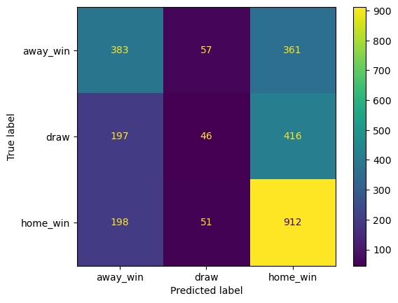
Default LightGBM confusion matrix

lgbm_default = lgb.LGBMClassifier()
lgbm_default.fit(X_all_train_std, y_all_train_encd)
lgbm_default_pred = lgbm_default.predict(X_all_test_std)

lgbm_default_cm = confusion_matrix(le.inverse_transform(y_all_test_encd), 
                                   le.inverse_transform(lgbm_default_pred))
cm_display = ConfusionMatrixDisplay(confusion_matrix = lgbm_default_cm, 
                                    display_labels = le.inverse_transform(lgbm_default.classes_))
cm_display.plot();    

print(classification_report(le.inverse_transform(y_all_test_encd), 
                            le.inverse_transform(lgbm_default_pred)))

              precision    recall  f1-score   support

    away_win       0.49      0.48      0.49       801
        draw       0.30      0.07      0.11       659
    home_win       0.54      0.79      0.64      1161

    accuracy                           0.51      2621
   macro avg       0.44      0.44      0.41      2621
weighted avg       0.46      0.51      0.46      2621

4. Hyperparameter tuning

4.1. Random forest

• Candidate hyperparameters are as follow:
  • n_estimators: 100, 300, 500, 1000
  • learning_rate: 1e-8 ~ 1
  • max_depth: 3 ~ 20
  • max_features: auto, sqrt, log2
  • min_samples_leaf: 1 ~ 10
  • min_samples_split: 2 ~ 10

def rf_objective(trial, X, y):
    param_grid = {
        "n_estimators": trial.suggest_categorical("n_estimators", [100, 300, 500, 1000]),
        "max_depth": trial.suggest_int("max_depth", 3, 20, step = 2),
        "max_features": trial.suggest_categorical("max_features", ["sqrt", "log2"]),
        "min_samples_leaf": trial.suggest_int("min_samples_leaf", 1, 10),
        "min_samples_split": trial.suggest_int("min_samples_split", 2, 10),
    }
    
    cv = StratifiedKFold(n_splits = 5, shuffle = True, random_state = 42)
    cv_scores = np.empty(5)
    
    for idx, (train_idx, test_idx) in enumerate(cv.split(X, y)):
        X_train, X_test = X.iloc[train_idx], X.iloc[test_idx]
        y_train, y_test = y[train_idx], y[test_idx]
        
        model = RandomForestClassifier(**param_grid, n_jobs = -1)
        model.fit(X_train, y_train)
          
        pred = model.predict(X_test)
        cv_scores[idx] = np.mean(pred == y_test)

    return np.mean(cv_scores)

rf_study = optuna.create_study(direction = "maximize", study_name = "RandomForest Classifier")
func = lambda trial: rf_objective(trial, X_all_train_std, y_all_train_encd)
rf_study.optimize(func, n_trials = 20)

• Best parameters are as follow:

rf_study.best_params

{'n_estimators': 300,
 'max_depth': 5,
 'max_features': 'sqrt',
 'min_samples_leaf': 7,
 'min_samples_split': 4}

• Let’s check the test accuracy with the best hyperparameters set.

rf_best = RandomForestClassifier(**rf_study.best_params)
rf_best.fit(X_all_train_std, y_all_train_encd)
rf_best_pred = rf_best.predict(X_all_test_std)
rf_best_accuracy = np.mean(rf_best_pred == y_all_test_encd)

print("Accuracy before tuning the hyperparameters: ", result_accuracy[result_accuracy.model_name == "Random Forest"]["All Variables"].values[0])
print("Accuracy after tuning the hyperparameters: ", rf_best_accuracy * 100)

Accuracy before tuning the hyperparameters:  52.003
Accuracy after tuning the hyperparameters:  52.04120564669973

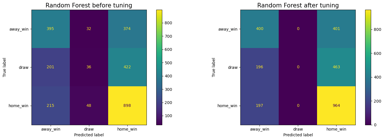
• Let’s check the confusion matrix of the tuned random forest model.

fig, axes = plt.subplots(1, 2, figsize = (15, 5))

# confusion matrix for the random forest with default hyperparameters

rf_default_display = ConfusionMatrixDisplay(confusion_matrix = rf_default_cm, 
                                            display_labels = le.inverse_transform(rf_default.classes_))

# confusion matrix for the random forest with the best hyperparameters

rf_tuned_cm = confusion_matrix(le.inverse_transform(y_all_test_encd), 
                               le.inverse_transform(rf_best_pred))
rf_best_display = ConfusionMatrixDisplay(confusion_matrix = rf_tuned_cm, 
                                    display_labels = le.inverse_transform(rf_best.classes_))

rf_default_display.plot(ax = axes[0])
axes[0].set_title("Random Forest before tuning", fontsize = 15)

rf_best_display.plot(ax = axes[1])
axes[1].set_title("Random Forest after tuning", fontsize = 15)

plt.tight_layout()

print("< Random Forest before tuning >")
print("")
print(classification_report(le.inverse_transform(y_all_test_encd), 
                            le.inverse_transform(rf_default_pred)))

print("")
print("< Random Forest after tuning >")
print("")
print(classification_report(le.inverse_transform(y_all_test_encd), 
                            le.inverse_transform(rf_best_pred)))

< Random Forest before tuning >

              precision    recall  f1-score   support

    away_win       0.49      0.49      0.49       801
        draw       0.31      0.05      0.09       659
    home_win       0.53      0.77      0.63      1161

    accuracy                           0.51      2621
   macro avg       0.44      0.44      0.40      2621
weighted avg       0.46      0.51      0.45      2621


< Random Forest after tuning >

              precision    recall  f1-score   support

    away_win       0.50      0.50      0.50       801
        draw       0.00      0.00      0.00       659
    home_win       0.53      0.83      0.65      1161

    accuracy                           0.52      2621
   macro avg       0.34      0.44      0.38      2621
weighted avg       0.39      0.52      0.44      2621

• Results for away_win and home_win have improved, but the model is struggling to predict the draw.

4.2. LightGBM

• Candidate hyperparameters are as follow:
  • learning_rate: 0.01 ~ 0.3
  • num_leaves: 20 ~ 3000 with step = 20
  • max_depth: 3 ~ 12
  • min_data_in_leaf: 200 ~ 10000 with step = 100
  • max_bing: 200 ~ 300
  • lambda_l1: 0 ~ 100 with step = 5
  • lambda_l2: 0 ~ 100 with step = 5
  • min_gain_to_split: 0 ~ 15
  • bagging_fraction: 0.2 ~ 0.95 with step = 0.1
  • feature_fraction: 0.2 ~ 0.95 with step = 0.1

def lgbm_objective(trial, X, y):
    param_grid = {
        "n_estimators": trial.suggest_categorical("n_estimators", [10000]),
        "learning_rate": trial.suggest_float("learning_rate", 0.01, 0.3),
        "num_leaves": trial.suggest_int("num_leaves", 20, 3000, step = 20),
        "max_depth": trial.suggest_int("max_depth", 3, 12),
        "min_data_in_leaf": trial.suggest_int("min_data_in_leaf", 200, 10000, step = 100),
        "max_bin": trial.suggest_int("max_bin", 200, 300),
        "lambda_l1": trial.suggest_int("lambda_l1", 0, 100, step = 5),
        "lambda_l2": trial.suggest_int("lambda_l2", 0, 100, step = 5),
        "min_gain_to_split": trial.suggest_float("min_gain_to_split", 0, 15),
        "bagging_fraction": trial.suggest_float(
            "bagging_fraction", 0.2, 0.95, step = 0.1
        ),
        "bagging_freq": trial.suggest_categorical("bagging_freq", [1]),
        "feature_fraction": trial.suggest_float(
            "feature_fraction", 0.2, 0.95, step = 0.1
        ),
        "silent": 1,
        "verbose": -1
    }
    
    cv = StratifiedKFold(n_splits = 5, shuffle = True, random_state = 42)
    cv_scores = np.empty(5)
    
    for idx, (train_idx, test_idx) in enumerate(cv.split(X, y)):
        X_train, X_test = X.iloc[train_idx], X.iloc[test_idx]
        y_train, y_test = y[train_idx], y[test_idx]

        model = lgb.LGBMClassifier(objective = "multiclass", num_class = 3, **param_grid, n_jobs = -1)
        model.fit(
            X_train,
            y_train,
            eval_set=[(X_test, y_test)],
            #eval_metric = accuracy_score,
            early_stopping_rounds = 100,
            # callbacks=[
            #     LightGBMPruningCallback(trial, accuracy_score)
            # ],  # Add a pruning callback
            verbose = -1
        )
        preds = model.predict(X_test)
        accuracy = np.mean(y_test == preds)
        cv_scores[idx] = accuracy

    return np.mean(cv_scores)

lgbm_study = optuna.create_study(direction = "maximize", study_name = "LightGBM Classifier")
func = lambda trial: lgbm_objective(trial, X_all_train_std, y_all_train_encd)
lgbm_study.optimize(func, n_trials = 100)

• Best parameters are as follow:

lgbm_study.best_params

{'n_estimators': 10000,
 'learning_rate': 0.29341244351241397,
 'num_leaves': 1560,
 'max_depth': 12,
 'min_data_in_leaf': 1800,
 'max_bin': 205,
 'lambda_l1': 20,
 'lambda_l2': 0,
 'min_gain_to_split': 12.558014144849205,
 'bagging_fraction': 0.8,
 'bagging_freq': 1,
 'feature_fraction': 0.30000000000000004}

lgb_best = lgb.LGBMClassifier(**lgbm_study.best_params, n_jobs = -1)
lgb_best.fit(X_all_train_std, y_all_train_encd)
lgb_best_pred = lgb_best.predict(X_all_test_std)
lgbm_best_accuracy = np.mean(lgb_best_pred == y_all_test_encd)

print("Accuracy before tuning the hyperparameters: ", result_accuracy[result_accuracy.model_name == "LightGBM"]["All Variables"].values[0])
print("Accuracy after tuning the hyperparameters: ", lgbm_best_accuracy * 100)

Accuracy before tuning the hyperparameters:  51.164
Accuracy after tuning the hyperparameters:  52.003052270125906

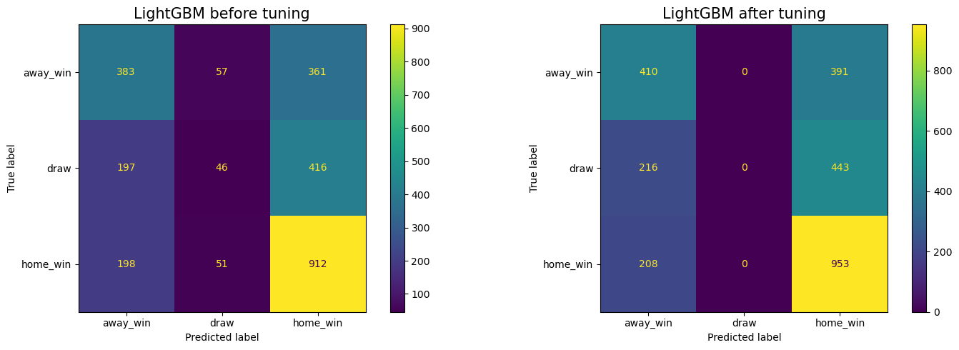
fig, axes = plt.subplots(1, 2, figsize = (15, 5))

# confusion matrix for the lgbm with default hyperparameters

lgbm_default_display = ConfusionMatrixDisplay(confusion_matrix = lgbm_default_cm, 
                                              display_labels = le.inverse_transform(lgbm_default.classes_))

# confusion matrix for the lgbm with the best hyperparameters

lgbm_tuned_cm = confusion_matrix(le.inverse_transform(y_all_test_encd), 
                                 le.inverse_transform(lgb_best_pred))
lgbm_best_display = ConfusionMatrixDisplay(confusion_matrix = lgbm_tuned_cm, 
                                           display_labels = le.inverse_transform(lgb_best.classes_))

lgbm_default_display.plot(ax = axes[0])
axes[0].set_title("LightGBM before tuning", fontsize = 15)

lgbm_best_display.plot(ax = axes[1])
axes[1].set_title("LightGBM after tuning", fontsize = 15)

plt.tight_layout()

print("< LightGBM before tuning >")
print("")
print(classification_report(le.inverse_transform(y_all_test_encd), 
                            le.inverse_transform(lgbm_default_pred)))

print("")
print("< LightGBM after tuning >")
print("")
print(classification_report(le.inverse_transform(y_all_test_encd), 
                            le.inverse_transform(lgb_best_pred)))

< LightGBM before tuning >

              precision    recall  f1-score   support

    away_win       0.49      0.48      0.49       801
        draw       0.30      0.07      0.11       659
    home_win       0.54      0.79      0.64      1161

    accuracy                           0.51      2621
   macro avg       0.44      0.44      0.41      2621
weighted avg       0.46      0.51      0.46      2621


< LightGBM after tuning >

              precision    recall  f1-score   support

    away_win       0.49      0.51      0.50       801
        draw       0.00      0.00      0.00       659
    home_win       0.53      0.82      0.65      1161

    accuracy                           0.52      2621
   macro avg       0.34      0.44      0.38      2621
weighted avg       0.39      0.52      0.44      2621

• Results for away_win and home_win have improved, but the LightGBM is also struggling to predict the draw.

5. Feature importance

• Let’s check the feature importance from the tuned random forest model based on feature permutation.

rf_best_params = {
    'n_estimators': 300,
    'max_depth': 5,
    'max_features': 'sqrt',
    'min_samples_leaf': 7,
    'min_samples_split': 4
}

rf_best = RandomForestClassifier(**rf_best_params)
rf_best.fit(X_all_train_std, y_all_train_encd)
rf_best_pred = rf_best.predict(X_all_test_std)
rf_best_accuracy = np.mean(rf_best_pred == y_all_test_encd)

result = permutation_importance(
    rf_best, X_all_test_std, y_all_test_encd, n_repeats=10, random_state=42, n_jobs=-1
)

rf_feature_imp_permutation =  pd.DataFrame(sorted(zip(result.importances_mean, col_names)), columns=['Value','Feature'])

plt.figure(figsize=(20, 10))
sns.barplot(x="Value", y="Feature", data = rf_feature_imp_permutation.sort_values("Value", ascending = False).head(50))
plt.title('Random Forest Features')
plt.tight_layout()
plt.show()

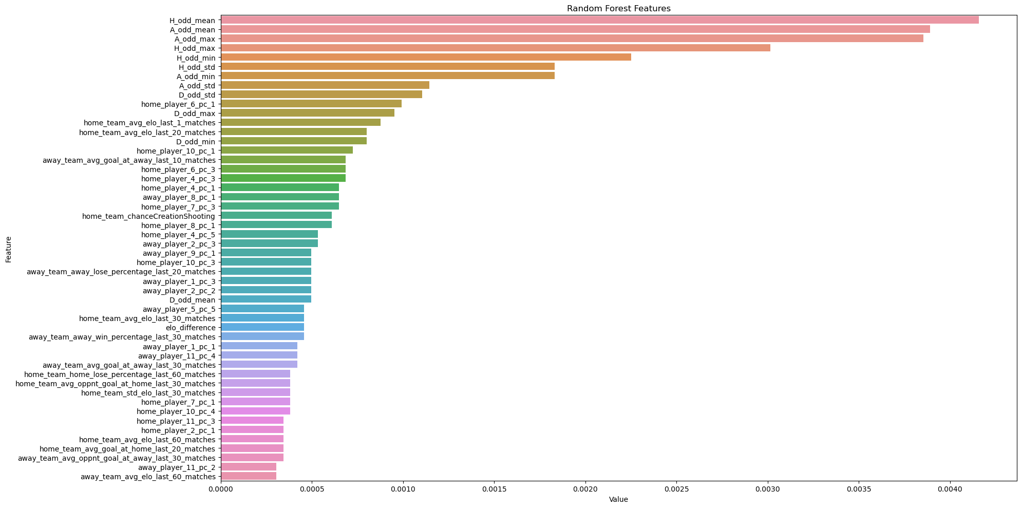
• Above plot shows top 50 most important features for predicting the match results.

• Let’s compare the distribution of the feature importance between different variable sets.

  • variable set 1: player attributes PC features
  • Variable set 2: betting information features
  • variable set 3: team attributes features
  • variable set 4: goal and win percentage rolling features
  • variable set 5: each team’s Elo rating

player_attr_pc_vars = df_match_player_attr_pcs.columns
bet_stat_vars = df_match_betting_stat.columns
team_attr_vars = df_match_team_num_attr.columns
team_rolling_vars = df_team_win_goal_rolling_features.columns
elo_vars = df_match_elo.columns

rf_feature_imp_permutation.loc[rf_feature_imp_permutation.Feature.isin(player_attr_pc_vars), "feature_set"] = f"Player attribute PC variables (#: {len(player_attr_pc_vars) - 1})"
rf_feature_imp_permutation.loc[rf_feature_imp_permutation.Feature.isin(bet_stat_vars), "feature_set"] = f"Betting odds statistics variables (#: {len(bet_stat_vars) - 1})"
rf_feature_imp_permutation.loc[rf_feature_imp_permutation.Feature.isin(team_attr_vars), "feature_set"] = f"Team attribute variables (#: {len(team_attr_vars) - 1})"
rf_feature_imp_permutation.loc[rf_feature_imp_permutation.Feature.isin(team_rolling_vars), "feature_set"] = f"Team's recent average goal and win percentage variables (#: {len(team_rolling_vars) - 1})"
rf_feature_imp_permutation.loc[rf_feature_imp_permutation.Feature.isin(elo_vars), "feature_set"] = f"Team's recent Elo variables (#: {len(elo_vars) - 1})"

plt.figure(figsize = (12, 5))
sns.boxplot(data = rf_feature_imp_permutation, x = "Value", y = "feature_set")
plt.xlabel("Feature importance", fontsize = 12)
plt.ylabel("Feature sets", fontsize = 12)
plt.title("Feature importance distribution from different feature sets", fontsize = 15)

Text(0.5, 1.0, 'Feature importance distribution from different feature sets')

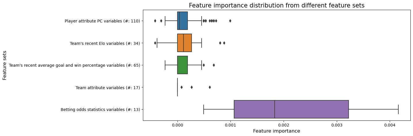
• The betting odds statistics variables shows the highest importance among different feature sets.
• Team attribute variables have the lowest feature importance.
• The remaining three variable sets show similar importance.

5.1. Betting odds statistics variables

• Betting odds statistics can be subdivided into:
  • home win, away win, and draw
  • mean, max, min, std

betting_importance = rf_feature_imp_permutation[rf_feature_imp_permutation.feature_set == "Betting odds statistics variables (#: 13)"]
betting_importance["home_away"] = betting_importance.Feature.str.split("_").str[0]
betting_importance["statistics"] = betting_importance.Feature.str.split("_").str[2]

betting_importance.sort_values("Value", ascending = False)

	Value	Feature	feature_set	home_away	statistics
234	0.004159	H_odd_mean	Betting odds statistics variables (#: 13)	H	mean
233	0.003892	A_odd_mean	Betting odds statistics variables (#: 13)	A	mean
232	0.003853	A_odd_max	Betting odds statistics variables (#: 13)	A	max
231	0.003014	H_odd_max	Betting odds statistics variables (#: 13)	H	max
230	0.002251	H_odd_min	Betting odds statistics variables (#: 13)	H	min
229	0.001831	H_odd_std	Betting odds statistics variables (#: 13)	H	std
228	0.001831	A_odd_min	Betting odds statistics variables (#: 13)	A	min
227	0.001145	A_odd_std	Betting odds statistics variables (#: 13)	A	std
226	0.001106	D_odd_std	Betting odds statistics variables (#: 13)	D	std
224	0.000954	D_odd_max	Betting odds statistics variables (#: 13)	D	max
221	0.000801	D_odd_min	Betting odds statistics variables (#: 13)	D	min
204	0.000496	D_odd_mean	Betting odds statistics variables (#: 13)	D	mean

• The importance of variables for home and away were high, and the importance of variables for draw were low.
• The importance of variables related to mean and max were high.

5.2. Team’s recent Elo variables

• Elo rating related variables can be subdivided into:
  • home team, away team
  • average, std
  • recent 1, 3, 5, 10, 20, 30, 60, 90 matches

elo_importance = rf_feature_imp_permutation[rf_feature_imp_permutation.feature_set == "Team's recent Elo variables (#: 34)"]

elo_importance["home_away"] = elo_importance.Feature.str.split("_").str[0]
elo_importance["statistics"] = elo_importance.Feature.str.split("_").str[2]
elo_importance["matches"] = elo_importance.Feature.str.split("_").str[5]

elo_importance.groupby("home_away").Value.mean().reset_index()

	home_away	Value
0	away	0.000057
1	elo	0.000458
2	home	0.000210