2 - 4) EDA - Match in-game shot information
import numpy as np
import pandas as pd

import sqlite3 as sql

import matplotlib.pyplot as plt
import matplotlib.patches as mpatches
import seaborn as sns
import missingno as msno

from utils import my_histogram
import warnings
warnings.filterwarnings('ignore')
pd.set_option('display.max_columns', None)
con = sql.connect("../data/database.sqlite")
df_match_ingame_shot = pd.read_csv("../data/df_match_ingame_shot.csv")
df_match_basic = pd.read_csv("../data/df_match_basic.csv")
- Let’s analyze the goal and shot information from df_match_ingame_shot and df_match_basic table.
df_match_ingame_shot
| match_api_id | event_id | elapsed | team_api_id | category | type | subtype | player1_api_id | player2_api_id | |
|---|---|---|---|---|---|---|---|---|---|
| 0 | 489042 | 378998 | 22 | 10261.0 | goal | n | header | 37799.0 | 38807.0 |
| 1 | 489042 | 379019 | 24 | 10260.0 | goal | n | shot | 24148.0 | 24154.0 |
| 2 | 489043 | 375546 | 4 | 9825.0 | goal | n | shot | 26181.0 | 39297.0 |
| 3 | 489044 | 378041 | 83 | 8650.0 | goal | n | distance | 30853.0 | 30889.0 |
| 4 | 489045 | 376060 | 4 | 8654.0 | goal | n | shot | 23139.0 | 36394.0 |
| ... | ... | ... | ... | ... | ... | ... | ... | ... | ... |
| 229033 | 2030171 | 4940379 | 19 | 8370.0 | shot | shotoff | NaN | 36130.0 | NaN |
| 229034 | 2030171 | 4940624 | 44 | 8370.0 | shot | shotoff | NaN | 34104.0 | NaN |
| 229035 | 2030171 | 4940738 | 49 | 8558.0 | shot | shotoff | NaN | 107930.0 | NaN |
| 229036 | 2030171 | 4940963 | 71 | 8370.0 | shot | shotoff | NaN | 210065.0 | NaN |
| 229037 | 2030171 | 4941072 | 83 | 8558.0 | shot | shotoff | NaN | 629579.0 | NaN |
229038 rows × 9 columns
df_match_basic
| match_api_id | country_id | league_id | season | stage | match_date | home_team_api_id | away_team_api_id | home_team_goal | away_team_goal | match_result | |
|---|---|---|---|---|---|---|---|---|---|---|---|
| 0 | 492473 | 1 | 1 | 2008/2009 | 1 | 2008-08-17 | 9987 | 9993 | 1 | 1 | draw |
| 1 | 492474 | 1 | 1 | 2008/2009 | 1 | 2008-08-16 | 10000 | 9994 | 0 | 0 | draw |
| 2 | 492475 | 1 | 1 | 2008/2009 | 1 | 2008-08-16 | 9984 | 8635 | 0 | 3 | away_win |
| 3 | 492476 | 1 | 1 | 2008/2009 | 1 | 2008-08-17 | 9991 | 9998 | 5 | 0 | home_win |
| 4 | 492477 | 1 | 1 | 2008/2009 | 1 | 2008-08-16 | 7947 | 9985 | 1 | 3 | away_win |
| ... | ... | ... | ... | ... | ... | ... | ... | ... | ... | ... | ... |
| 25974 | 1992091 | 24558 | 24558 | 2015/2016 | 9 | 2015-09-22 | 10190 | 10191 | 1 | 0 | home_win |
| 25975 | 1992092 | 24558 | 24558 | 2015/2016 | 9 | 2015-09-23 | 9824 | 10199 | 1 | 2 | away_win |
| 25976 | 1992093 | 24558 | 24558 | 2015/2016 | 9 | 2015-09-23 | 9956 | 10179 | 2 | 0 | home_win |
| 25977 | 1992094 | 24558 | 24558 | 2015/2016 | 9 | 2015-09-22 | 7896 | 10243 | 0 | 0 | draw |
| 25978 | 1992095 | 24558 | 24558 | 2015/2016 | 9 | 2015-09-23 | 10192 | 9931 | 4 | 3 | home_win |
25979 rows × 11 columns
- Combine the home team id, away team id, match date, match result, and season information to the df_match_ingame_shot table.
home_info = df_match_basic[["match_api_id", "home_team_api_id", "match_date", "match_result", "season"]].rename(columns = {"home_team_api_id": "team_api_id"})
home_info["home_away"] = "home"
away_info = df_match_basic[["match_api_id", "away_team_api_id", "match_date", "match_result", "season"]].rename(columns = {"away_team_api_id": "team_api_id"})
away_info["home_away"] = "away"
home_away_info = pd.concat([home_info, away_info], axis = 0)
df_match_ingame_shot = df_match_ingame_shot.merge(home_away_info, how = "left", on = ["match_api_id", "team_api_id"])
df_match_ingame_shot
| match_api_id | event_id | elapsed | team_api_id | category | type | subtype | player1_api_id | player2_api_id | match_date | match_result | season | home_away | |
|---|---|---|---|---|---|---|---|---|---|---|---|---|---|
| 0 | 489042 | 378998 | 22 | 10261.0 | goal | n | header | 37799.0 | 38807.0 | 2008-08-17 | draw | 2008/2009 | away |
| 1 | 489042 | 379019 | 24 | 10260.0 | goal | n | shot | 24148.0 | 24154.0 | 2008-08-17 | draw | 2008/2009 | home |
| 2 | 489043 | 375546 | 4 | 9825.0 | goal | n | shot | 26181.0 | 39297.0 | 2008-08-16 | home_win | 2008/2009 | home |
| 3 | 489044 | 378041 | 83 | 8650.0 | goal | n | distance | 30853.0 | 30889.0 | 2008-08-16 | away_win | 2008/2009 | away |
| 4 | 489045 | 376060 | 4 | 8654.0 | goal | n | shot | 23139.0 | 36394.0 | 2008-08-16 | home_win | 2008/2009 | home |
| ... | ... | ... | ... | ... | ... | ... | ... | ... | ... | ... | ... | ... | ... |
| 229033 | 2030171 | 4940379 | 19 | 8370.0 | shot | shotoff | NaN | 36130.0 | NaN | 2015-10-23 | home_win | 2015/2016 | home |
| 229034 | 2030171 | 4940624 | 44 | 8370.0 | shot | shotoff | NaN | 34104.0 | NaN | 2015-10-23 | home_win | 2015/2016 | home |
| 229035 | 2030171 | 4940738 | 49 | 8558.0 | shot | shotoff | NaN | 107930.0 | NaN | 2015-10-23 | home_win | 2015/2016 | away |
| 229036 | 2030171 | 4940963 | 71 | 8370.0 | shot | shotoff | NaN | 210065.0 | NaN | 2015-10-23 | home_win | 2015/2016 | home |
| 229037 | 2030171 | 4941072 | 83 | 8558.0 | shot | shotoff | NaN | 629579.0 | NaN | 2015-10-23 | home_win | 2015/2016 | away |
229038 rows × 13 columns
- Combine the league name to the df_match_ingame_shot table.
org_league = pd.read_sql(
    "select * from League", con
    )
df_match_ingame_shot = df_match_ingame_shot.merge(df_match_basic[["match_api_id", "league_id"]], how = "left", on = "match_api_id")
df_match_ingame_shot = df_match_ingame_shot.merge(org_league.rename(columns = {"id" : "league_id", "name": "league_name"}),
                                                            how = "left", on = "league_id")
df_match_ingame_shot.drop(["league_id", "country_id"], axis = 1, inplace = True)
df_match_ingame_shot
| match_api_id | event_id | elapsed | team_api_id | category | type | subtype | player1_api_id | player2_api_id | match_date | match_result | season | home_away | league_name | |
|---|---|---|---|---|---|---|---|---|---|---|---|---|---|---|
| 0 | 489042 | 378998 | 22 | 10261.0 | goal | n | header | 37799.0 | 38807.0 | 2008-08-17 | draw | 2008/2009 | away | England Premier League |
| 1 | 489042 | 379019 | 24 | 10260.0 | goal | n | shot | 24148.0 | 24154.0 | 2008-08-17 | draw | 2008/2009 | home | England Premier League |
| 2 | 489043 | 375546 | 4 | 9825.0 | goal | n | shot | 26181.0 | 39297.0 | 2008-08-16 | home_win | 2008/2009 | home | England Premier League |
| 3 | 489044 | 378041 | 83 | 8650.0 | goal | n | distance | 30853.0 | 30889.0 | 2008-08-16 | away_win | 2008/2009 | away | England Premier League |
| 4 | 489045 | 376060 | 4 | 8654.0 | goal | n | shot | 23139.0 | 36394.0 | 2008-08-16 | home_win | 2008/2009 | home | England Premier League |
| ... | ... | ... | ... | ... | ... | ... | ... | ... | ... | ... | ... | ... | ... | ... |
| 229033 | 2030171 | 4940379 | 19 | 8370.0 | shot | shotoff | NaN | 36130.0 | NaN | 2015-10-23 | home_win | 2015/2016 | home | Spain LIGA BBVA |
| 229034 | 2030171 | 4940624 | 44 | 8370.0 | shot | shotoff | NaN | 34104.0 | NaN | 2015-10-23 | home_win | 2015/2016 | home | Spain LIGA BBVA |
| 229035 | 2030171 | 4940738 | 49 | 8558.0 | shot | shotoff | NaN | 107930.0 | NaN | 2015-10-23 | home_win | 2015/2016 | away | Spain LIGA BBVA |
| 229036 | 2030171 | 4940963 | 71 | 8370.0 | shot | shotoff | NaN | 210065.0 | NaN | 2015-10-23 | home_win | 2015/2016 | home | Spain LIGA BBVA |
| 229037 | 2030171 | 4941072 | 83 | 8558.0 | shot | shotoff | NaN | 629579.0 | NaN | 2015-10-23 | home_win | 2015/2016 | away | Spain LIGA BBVA |
229038 rows × 14 columns
- Combine the league name to the df_match_basic table.
df_match_basic = df_match_basic.merge(org_league.drop("country_id", axis = 1).rename(columns = {"id" : "league_id", "name": "league_name"}),
                                                      how = "left", on = "league_id")
df_match_basic.drop(["league_id", "country_id"], axis = 1, inplace = True)
df_match_basic
| match_api_id | season | stage | match_date | home_team_api_id | away_team_api_id | home_team_goal | away_team_goal | match_result | league_name | |
|---|---|---|---|---|---|---|---|---|---|---|
| 0 | 492473 | 2008/2009 | 1 | 2008-08-17 | 9987 | 9993 | 1 | 1 | draw | Belgium Jupiler League |
| 1 | 492474 | 2008/2009 | 1 | 2008-08-16 | 10000 | 9994 | 0 | 0 | draw | Belgium Jupiler League |
| 2 | 492475 | 2008/2009 | 1 | 2008-08-16 | 9984 | 8635 | 0 | 3 | away_win | Belgium Jupiler League |
| 3 | 492476 | 2008/2009 | 1 | 2008-08-17 | 9991 | 9998 | 5 | 0 | home_win | Belgium Jupiler League |
| 4 | 492477 | 2008/2009 | 1 | 2008-08-16 | 7947 | 9985 | 1 | 3 | away_win | Belgium Jupiler League |
| ... | ... | ... | ... | ... | ... | ... | ... | ... | ... | ... |
| 25974 | 1992091 | 2015/2016 | 9 | 2015-09-22 | 10190 | 10191 | 1 | 0 | home_win | Switzerland Super League |
| 25975 | 1992092 | 2015/2016 | 9 | 2015-09-23 | 9824 | 10199 | 1 | 2 | away_win | Switzerland Super League |
| 25976 | 1992093 | 2015/2016 | 9 | 2015-09-23 | 9956 | 10179 | 2 | 0 | home_win | Switzerland Super League |
| 25977 | 1992094 | 2015/2016 | 9 | 2015-09-22 | 7896 | 10243 | 0 | 0 | draw | Switzerland Super League |
| 25978 | 1992095 | 2015/2016 | 9 | 2015-09-23 | 10192 | 9931 | 4 | 3 | home_win | Switzerland Super League |
25979 rows × 10 columns
1. Goal
df_match_ingame_shot_goal = df_match_ingame_shot[df_match_ingame_shot.category == "goal"]
1.1. Goal trend
Q. Is there any goal trend change over the seasons?
goals_trend = df_match_basic.groupby(["league_name", "season"]).mean()[["home_team_goal", "away_team_goal"]].reset_index()
fig, axes = plt.subplots(4, 3, figsize = (20, 15))

for i, league in enumerate(goals_trend.league_name.unique()):
    home = goals_trend.loc[goals_trend.league_name == league, ["league_name", "season", "home_team_goal"]].rename(columns = {"home_team_goal" : "goals"})
    home["home_away"] = "home"

    away = goals_trend.loc[goals_trend.league_name == league, ["league_name", "season", "away_team_goal"]].rename(columns = {"away_team_goal" : "goals"})
    away["home_away"] = "away"

    home_m_away = home.copy()
    home_m_away["goals"] = home.goals - away.goals
    home_m_away["home_away"] = "home goals - away goals"

    home_away = pd.concat([home, away, home_m_away], axis = 0)

    sns.lineplot(data = home_away, x = "season", y = "goals", hue = "home_away", marker = "o", ax = axes[i // 3, i % 3])

    axes[i // 3, i % 3].set_xlabel(" ", fontsize = 10)
    axes[i // 3, i % 3].set_ylabel(" ", fontsize = 10)
    axes[i // 3, i % 3].set_title(f"{league} goals trend", fontsize = 15)
    axes[i // 3, i % 3].tick_params(axis='x', labelrotation = 90)

plt.tight_layout()
- Home team scores more goals than away team in all leagues.
- The gap between the average number of home goals and the average number of away goals has remained similar across all seasons from the each league.
$\quad \rightarrow$ Since season has no effect in the goal trend, let’s check the goal distribution without considering the season.
1.2. Goal distribution
- The number of goals has the most direct effect on winning or losing. If a team score more goals and get less, the team can win the game.
- If we can identify the characteristics of a team that scores a lot of goals and a team that scores few goals, we will have an advantage in predicting the match result.
Q. How many more goals did the winning team score than the losing team?
plt.figure(figsize = (15, 6))
sns.countplot(x = abs(df_match_basic[df_match_basic.match_result != "draw"].home_team_goal -
                      df_match_basic[df_match_basic.match_result != "draw"].away_team_goal))
plt.title("Difference of number of goals between winning team and losing tema", fontsize = 20)
plt.xlabel("Goal difference", fontsize = 13)
plt.ylabel("Count", fontsize = 13)
Text(0, 0.5, 'Count')
- Almost half of the matches are won by a difference of only one goal.
Q. The difference of number of goals between home and away team.
plt.figure(figsize = (15, 6))
sns.countplot(x = df_match_basic.home_team_goal - df_match_basic.away_team_goal)
plt.title("Difference of number of goals between home team and away team", fontsize = 20)
plt.xlabel("Goal difference", fontsize = 13)
plt.ylabel("Count", fontsize = 13)
Text(0, 0.5, 'Count')
- The side larger than 0 in the distribution is slightly thicker than the smaller side.
- That is, home team usually scores more goals than the away team.
Q. What is the difference between home and away team win rates?
df_match_basic.match_result.value_counts()
home_win    11917
away_win     7466
draw         6596
Name: match_result, dtype: int64
sns.countplot(x = df_match_basic.match_result,
              order = ["home_win", "draw", "away_win"])
plt.xlabel("Match result", fontsize = 15)
plt.ylabel("Count", fontsize = 15)
Text(0, 0.5, 'Count')
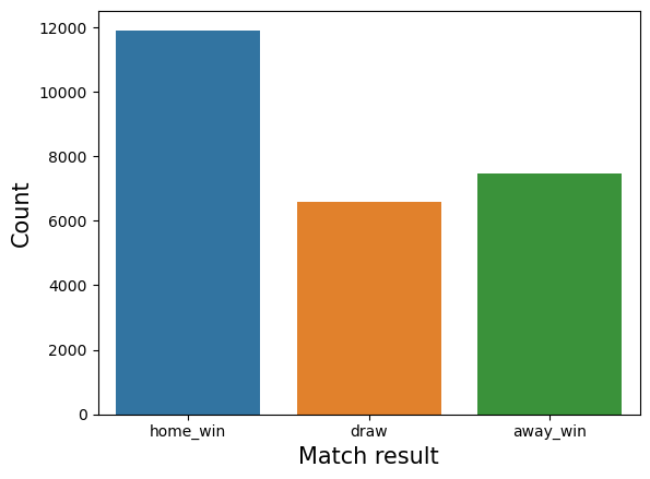
- Out of a total of 25979 matches
- About 45% (11917 / 25979) were won by the home team
- About 25% (6596 / 25979) were draw
- About 29% (7466 / 25979) were won by the away team
$\color{magenta} \quad \rightarrow$ This percentage can be used as a baseline accuracy later.
Q. Is there a difference in the distribution of home and away team goals by league?
df_match_basic.groupby("league_name").home_team_goal.describe()
| count | mean | std | min | 25% | 50% | 75% | max | |
|---|---|---|---|---|---|---|---|---|
| league_name | ||||||||
| Belgium Jupiler League | 1728.0 | 1.609375 | 1.293458 | 0.0 | 1.0 | 1.0 | 2.0 | 7.0 |
| England Premier League | 3040.0 | 1.550987 | 1.311615 | 0.0 | 1.0 | 1.0 | 2.0 | 9.0 |
| France Ligue 1 | 3040.0 | 1.402961 | 1.170743 | 0.0 | 1.0 | 1.0 | 2.0 | 6.0 |
| Germany 1. Bundesliga | 2448.0 | 1.626634 | 1.339529 | 0.0 | 1.0 | 1.0 | 2.0 | 9.0 |
| Italy Serie A | 3017.0 | 1.500829 | 1.221797 | 0.0 | 1.0 | 1.0 | 2.0 | 7.0 |
| Netherlands Eredivisie | 2448.0 | 1.779820 | 1.405274 | 0.0 | 1.0 | 2.0 | 3.0 | 10.0 |
| Poland Ekstraklasa | 1920.0 | 1.394792 | 1.183249 | 0.0 | 0.0 | 1.0 | 2.0 | 6.0 |
| Portugal Liga ZON Sagres | 2052.0 | 1.408382 | 1.226192 | 0.0 | 0.0 | 1.0 | 2.0 | 8.0 |
| Scotland Premier League | 1824.0 | 1.429276 | 1.294928 | 0.0 | 0.0 | 1.0 | 2.0 | 9.0 |
| Spain LIGA BBVA | 3040.0 | 1.631250 | 1.388339 | 0.0 | 1.0 | 1.0 | 2.0 | 10.0 |
| Switzerland Super League | 1422.0 | 1.663150 | 1.363970 | 0.0 | 1.0 | 1.0 | 3.0 | 7.0 |
fig, axes = plt.subplots(1, 2, figsize = (20, 7), sharey = True)

sns.boxplot(data = df_match_basic, x = "home_team_goal", y = "league_name", showfliers = False, ax = axes[0])
axes[0].set_xlabel("goals", fontsize = 15)
axes[0].set_ylabel("League", fontsize = 15)
axes[0].set_title("Home team goals distribution", fontsize = 20)

sns.barplot(df_match_basic.groupby("league_name").home_team_goal.describe().reset_index(), x = "mean", y = "league_name")
axes[1].set_xlabel("goals", fontsize = 15)
axes[1].set_ylabel("League", fontsize = 15)
axes[1].set_title("Home team average goals per game", fontsize = 20)
Text(0.5, 1.0, 'Home team average goals per game')
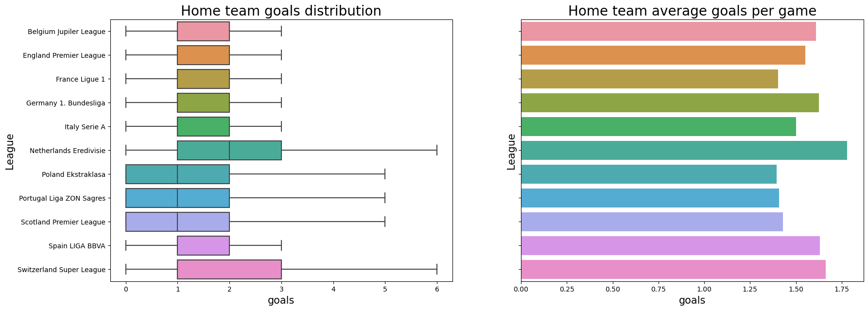
- Looking at the distribution of the number of home team goals by league over 8 seasons, it can be seen that the Dutch and Swiss leagues have more home team goals than other leagues.
- Average Home team goals per game are around 1.5 across all leagues.
- In the case of the France, Poland, Portugal, and Scotland, home team average goals per game are slightly lower than other leagues.
- In the case of the Netherland, home team average goals per game are slightly higher than other leagues.
df_match_basic.groupby("league_name").away_team_goal.describe()
| count | mean | std | min | 25% | 50% | 75% | max | |
|---|---|---|---|---|---|---|---|---|
| league_name | ||||||||
| Belgium Jupiler League | 1728.0 | 1.192130 | 1.125123 | 0.0 | 0.0 | 1.0 | 2.0 | 7.0 |
| England Premier League | 3040.0 | 1.159539 | 1.144629 | 0.0 | 0.0 | 1.0 | 2.0 | 6.0 |
| France Ligue 1 | 3040.0 | 1.040132 | 1.059765 | 0.0 | 0.0 | 1.0 | 2.0 | 9.0 |
| Germany 1. Bundesliga | 2448.0 | 1.274918 | 1.200392 | 0.0 | 0.0 | 1.0 | 2.0 | 8.0 |
| Italy Serie A | 3017.0 | 1.116009 | 1.078392 | 0.0 | 0.0 | 1.0 | 2.0 | 7.0 |
| Netherlands Eredivisie | 2448.0 | 1.301062 | 1.240430 | 0.0 | 0.0 | 1.0 | 2.0 | 6.0 |
| Poland Ekstraklasa | 1920.0 | 1.030208 | 1.046159 | 0.0 | 0.0 | 1.0 | 2.0 | 6.0 |
| Portugal Liga ZON Sagres | 2052.0 | 1.126218 | 1.155469 | 0.0 | 0.0 | 1.0 | 2.0 | 6.0 |
| Scotland Premier League | 1824.0 | 1.204496 | 1.151384 | 0.0 | 0.0 | 1.0 | 2.0 | 6.0 |
| Spain LIGA BBVA | 3040.0 | 1.135855 | 1.161079 | 0.0 | 0.0 | 1.0 | 2.0 | 8.0 |
| Switzerland Super League | 1422.0 | 1.266526 | 1.176233 | 0.0 | 0.0 | 1.0 | 2.0 | 7.0 |
fig, axes = plt.subplots(1, 2, figsize = (20, 7), sharey = True)

sns.boxplot(data = df_match_basic, x = "away_team_goal", y = "league_name", showfliers = False, ax = axes[0])
axes[0].set_xlabel("goals", fontsize = 15)
axes[0].set_ylabel("League", fontsize = 15)
axes[0].set_title("Away team goals distribution", fontsize = 20)

sns.barplot(df_match_basic.groupby("league_name").away_team_goal.describe().reset_index(), x = "mean", y = "league_name")
axes[1].set_xlabel("goals", fontsize = 15)
axes[1].set_ylabel("League", fontsize = 15)
axes[1].set_title("Away team average goals per game", fontsize = 20)

plt.tight_layout()
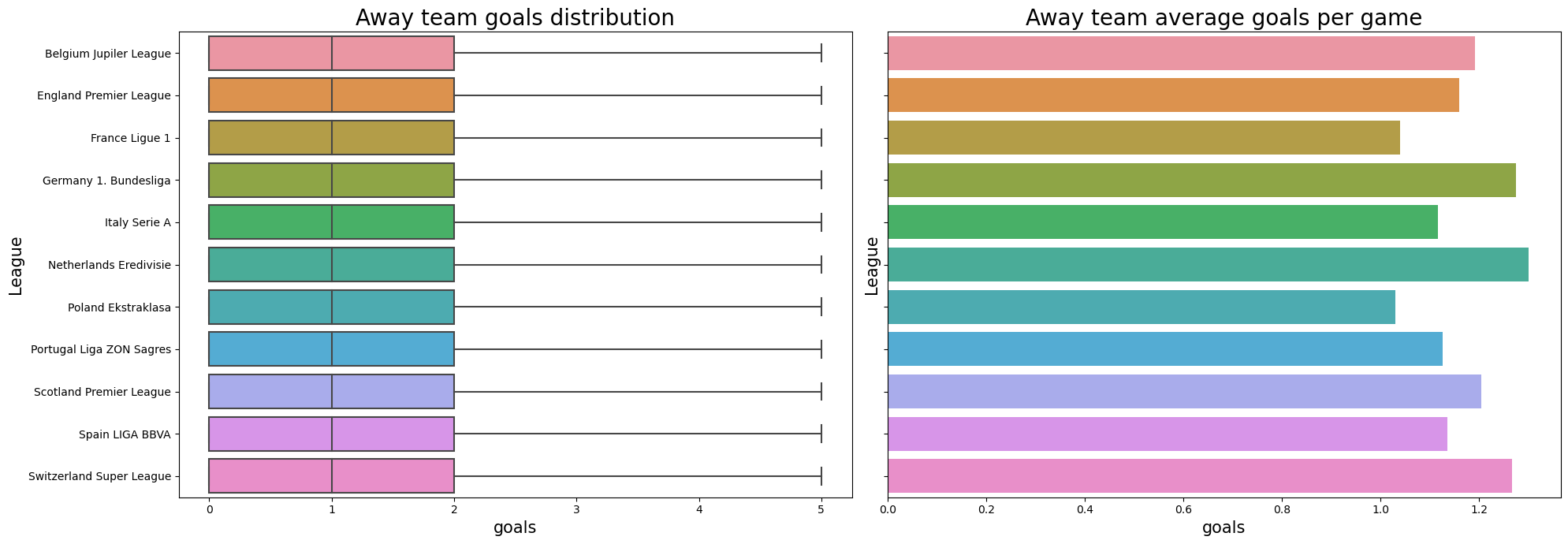
- The away team’s goals distribution over the eight seasons shows a nearly identical distribution across all leagues compared to the home team’s goals distributions.
- Away teams score around 1.1 goals per game on average across all leagues.
- In the case of the France and the Poland, away team average goals per game are slightly lower than other leagues.
-
In the case of the Germany, Netherlands, and Switzeland, away team average goals per game are slightly higher than other leagues.
- Average home and away team goals per game vary by league.
$\color{magenta} \quad \rightarrow$ There is a difference in the average goals of home and away teams in each league, so it is a good idea to try fitting our model differently for each league later.
Q. What is the difference between home and away team win rates between leagues ?
df_match_result_pivot = df_match_basic.pivot_table(index = "league_name", columns = "match_result", values = "stage", aggfunc = "count")
df_match_result_pivot["sum"] = df_match_result_pivot.sum(axis = 1)

match_result_prop = df_match_result_pivot[["home_win", "away_win", "draw"]].divide(df_match_result_pivot["sum"], axis = 0).multiply(100)
ax = match_result_prop.plot.barh(stacked = True, figsize = (10, 8), width = 0.75, edgecolor = 'w')
ax.legend(['Home Team','Away Team','Draw'], bbox_to_anchor = (1.2, 1), loc = 'upper right')
plt.title('Probability of match result by league', fontsize = 20)
plt.xlabel('Proportion',fontsize = 15)
plt.ylabel('Leagues', fontsize = 15)
plt.xticks(fontsize = 12)
plt.yticks(fontsize = 12)

for  i, j in enumerate(match_result_prop.index):
    plt.text(match_result_prop.loc[j, 'home_win']/2, i, str(round(match_result_prop.loc[j, 'home_win'], 2)) + ' %', fontsize = 12)
    plt.text(match_result_prop.loc[j, 'home_win'] + match_result_prop.loc[j,'away_win']/3, i, str(round(match_result_prop.loc[j,'away_win'], 2)) + ' %',fontsize = 12)
    plt.text(match_result_prop.loc[j, 'home_win'] + match_result_prop.loc[j,'away_win']+ match_result_prop.loc[j, 'draw']/2, i, str(round(match_result_prop.loc[j, 'draw'], 2)) + '%', fontsize = 12)
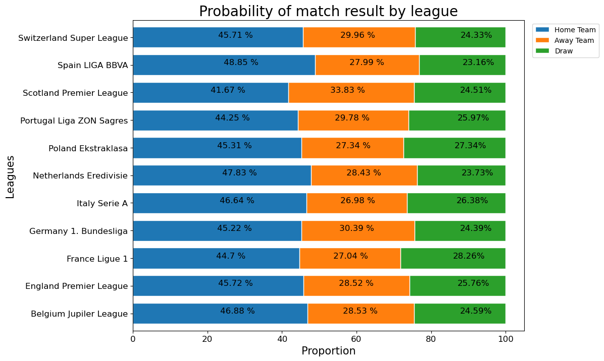
- The overall tendency for the home team to have the highest win rate and the lowest draw rate is similar across leagues.
- However, there are some differences in the detailed ratio.
$\color{magenta} \quad \rightarrow$ This league-specific ratios can later be used as the baseline accuracy for each league when fitting the model for each league.
Q. How strong is the relationship between home and away average goals and wins ?
- Usually, the home team scores more goals and the away team scores fewer goals, so the home team has a higher win rate.
-
It is important for us to predict in which matches the home team will lose, the away team will win, and neither team will win.
- So let’s try to figure out the relationship between how many goals are scored at home & away and the winning percentage.
df_team = pd.read_csv("../data/df_team.csv")
distinct_team = df_team[["team_api_id", "team_long_name"]].drop_duplicates()
goal_match_result_info = distinct_team.merge(df_match_basic.groupby("home_team_api_id").mean().home_team_goal.reset_index().rename(columns = {"home_team_api_id" : "team_api_id",
                                                                                                 "home_team_goal" : "home_avg_goal"}),
                                             how = "left", on = "team_api_id")
goal_match_result_info = goal_match_result_info.merge(df_match_basic.groupby("home_team_api_id").mean().away_team_goal.reset_index().rename(columns = {"home_team_api_id" : "team_api_id",
                                                                                                 "away_team_goal" : "home_opponent_avg_goal"}),
                                                      how = "left", on = "team_api_id")
goal_match_result_info = goal_match_result_info.merge(df_match_basic.groupby("away_team_api_id").mean().away_team_goal.reset_index().rename(columns = {"away_team_api_id" : "team_api_id",
                                                                                                 "away_team_goal" : "away_avg_goal"}),
                                                      how = "left", on = "team_api_id")
goal_match_result_info = goal_match_result_info.merge(df_match_basic.groupby("away_team_api_id").mean().home_team_goal.reset_index().rename(columns = {"away_team_api_id" : "team_api_id",
                                                                                                 "home_team_goal" : "away_opponent_avg_goal"}),
                                                      how = "left", on = "team_api_id")
result_from_home = df_match_basic.groupby(["home_team_api_id", "match_result"]).count().match_api_id.reset_index() \
                                 .pivot_table(index = "home_team_api_id", columns = "match_result", values = "match_api_id").reset_index()
result_from_home = result_from_home.rename(columns = {"home_team_api_id" : "team_api_id", "home_win": "win_at_home",
                                                      "draw": "draw_at_home", "away_win": "lose_at_home"})
result_from_home["num_home_matches"] = result_from_home.win_at_home + result_from_home.draw_at_home + result_from_home.lose_at_home
result_from_home["win_at_home"] = result_from_home.win_at_home / result_from_home.num_home_matches
result_from_home["draw_at_home"] = result_from_home.draw_at_home / result_from_home.num_home_matches
result_from_home["lose_at_home"] = result_from_home.lose_at_home / result_from_home.num_home_matches
result_from_home.drop("num_home_matches", axis = 1, inplace = True)
result_from_away = df_match_basic.groupby(["away_team_api_id", "match_result"]).count().match_api_id.reset_index() \
                                 .pivot_table(index = "away_team_api_id", columns = "match_result", values = "match_api_id").reset_index()
result_from_away = df_match_basic.groupby(["away_team_api_id", "match_result"]).count().match_api_id.reset_index() \
                                 .pivot_table(index = "away_team_api_id", columns = "match_result", values = "match_api_id").reset_index()
result_from_away = result_from_away.rename(columns = {"away_team_api_id" : "team_api_id", "home_win": "lose_at_away",
                                                      "draw": "draw_at_away", "away_win": "win_at_away"})
result_from_away["num_away_matches"] = result_from_away.win_at_away + result_from_away.draw_at_away + result_from_away.lose_at_away
result_from_away["win_at_away"] = result_from_away.win_at_away / result_from_away.num_away_matches
result_from_away["draw_at_away"] = result_from_away.draw_at_away / result_from_away.num_away_matches
result_from_away["lose_at_away"] = result_from_away.lose_at_away / result_from_away.num_away_matches
result_from_away.drop("num_away_matches", axis = 1, inplace = True)
result_from_away
| match_result | team_api_id | win_at_away | draw_at_away | lose_at_away |
|---|---|---|---|---|
| 0 | 1601 | 0.316667 | 0.241667 | 0.441667 |
| 1 | 1773 | 0.133333 | 0.333333 | 0.533333 |
| 2 | 1957 | 0.200000 | 0.308333 | 0.491667 |
| 3 | 2033 | 0.173333 | 0.373333 | 0.453333 |
| 4 | 2182 | 0.416667 | 0.275000 | 0.308333 |
| ... | ... | ... | ... | ... |
| 294 | 158085 | 0.204082 | 0.367347 | 0.428571 |
| 295 | 177361 | 0.200000 | 0.333333 | 0.466667 |
| 296 | 188163 | 0.294118 | 0.117647 | 0.588235 |
| 297 | 208931 | 0.157895 | 0.315789 | 0.526316 |
| 298 | 274581 | 0.166667 | 0.233333 | 0.600000 |
299 rows × 4 columns
goal_match_result_info = goal_match_result_info.merge(result_from_home[["team_api_id", "win_at_home", "draw_at_home", "lose_at_home"]], how = "left", on = "team_api_id") \
                                               .merge(result_from_away[["team_api_id", "win_at_away", "draw_at_away", "lose_at_away"]], how = "left", on = "team_api_id")
goal_match_result_info
| team_api_id | team_long_name | home_avg_goal | home_opponent_avg_goal | away_avg_goal | away_opponent_avg_goal | win_at_home | draw_at_home | lose_at_home | win_at_away | draw_at_away | lose_at_away | |
|---|---|---|---|---|---|---|---|---|---|---|---|---|
| 0 | 9930 | FC Aarau | 1.236111 | 1.652778 | 0.888889 | 2.152778 | 0.347222 | 0.166667 | 0.486111 | 0.138889 | 0.305556 | 0.555556 |
| 1 | 8485 | Aberdeen | 1.223684 | 0.967105 | 1.177632 | 1.381579 | 0.440789 | 0.250000 | 0.309211 | 0.348684 | 0.243421 | 0.407895 |
| 2 | 8576 | AC Ajaccio | 1.122807 | 1.350877 | 0.912281 | 1.877193 | 0.280702 | 0.333333 | 0.385965 | 0.105263 | 0.368421 | 0.526316 |
| 3 | 8564 | Milan | 1.794702 | 0.847682 | 1.480263 | 1.210526 | 0.609272 | 0.225166 | 0.165563 | 0.407895 | 0.296053 | 0.296053 |
| 4 | 10215 | Académica de Coimbra | 1.096774 | 1.258065 | 0.838710 | 1.532258 | 0.282258 | 0.387097 | 0.330645 | 0.169355 | 0.274194 | 0.556452 |
| ... | ... | ... | ... | ... | ... | ... | ... | ... | ... | ... | ... | ... |
| 283 | 10192 | BSC Young Boys | 2.230769 | 1.160839 | 1.468531 | 1.447552 | 0.594406 | 0.237762 | 0.167832 | 0.398601 | 0.244755 | 0.356643 |
| 284 | 8021 | Zagłębie Lubin | 1.288889 | 1.200000 | 1.011111 | 1.377778 | 0.388889 | 0.300000 | 0.311111 | 0.266667 | 0.266667 | 0.466667 |
| 285 | 8394 | Real Zaragoza | 1.250000 | 1.328947 | 0.842105 | 1.828947 | 0.381579 | 0.223684 | 0.394737 | 0.184211 | 0.223684 | 0.592105 |
| 286 | 8027 | Zawisza Bydgoszcz | 1.433333 | 1.266667 | 1.066667 | 1.700000 | 0.433333 | 0.166667 | 0.400000 | 0.200000 | 0.300000 | 0.500000 |
| 287 | 10000 | SV Zulte-Waregem | 1.660377 | 1.273585 | 1.226415 | 1.367925 | 0.424528 | 0.301887 | 0.273585 | 0.311321 | 0.283019 | 0.405660 |
288 rows × 12 columns
target_team_api = goal_match_result_info.sort_values("win_at_home", ascending = False).iloc[:25].team_api_id
goal_match_result_info.loc[goal_match_result_info.team_api_id.isin(target_team_api), "home_win_class"] = "home_win_best_10%_teams"

target_team_api = goal_match_result_info.sort_values("win_at_home").iloc[:25].team_api_id
goal_match_result_info.loc[goal_match_result_info.team_api_id.isin(target_team_api), "home_win_class"] = "home_win_worst_10%_teams"

target_team_api = goal_match_result_info.sort_values("win_at_away", ascending = False).iloc[:25].team_api_id
goal_match_result_info.loc[goal_match_result_info.team_api_id.isin(target_team_api), "away_win_class"] = "away_win_best_10%_teams"

target_team_api = goal_match_result_info.sort_values("win_at_away").iloc[:25].team_api_id
goal_match_result_info.loc[goal_match_result_info.team_api_id.isin(target_team_api), "away_win_class"] = "away_win_worst_10%_teams"
goal_match_result_info
| team_api_id | team_long_name | home_avg_goal | home_opponent_avg_goal | away_avg_goal | away_opponent_avg_goal | win_at_home | draw_at_home | lose_at_home | win_at_away | draw_at_away | lose_at_away | home_win_class | away_win_class | |
|---|---|---|---|---|---|---|---|---|---|---|---|---|---|---|
| 0 | 9930 | FC Aarau | 1.236111 | 1.652778 | 0.888889 | 2.152778 | 0.347222 | 0.166667 | 0.486111 | 0.138889 | 0.305556 | 0.555556 | NaN | NaN |
| 1 | 8485 | Aberdeen | 1.223684 | 0.967105 | 1.177632 | 1.381579 | 0.440789 | 0.250000 | 0.309211 | 0.348684 | 0.243421 | 0.407895 | NaN | NaN |
| 2 | 8576 | AC Ajaccio | 1.122807 | 1.350877 | 0.912281 | 1.877193 | 0.280702 | 0.333333 | 0.385965 | 0.105263 | 0.368421 | 0.526316 | NaN | away_win_worst_10%_teams |
| 3 | 8564 | Milan | 1.794702 | 0.847682 | 1.480263 | 1.210526 | 0.609272 | 0.225166 | 0.165563 | 0.407895 | 0.296053 | 0.296053 | NaN | NaN |
| 4 | 10215 | Académica de Coimbra | 1.096774 | 1.258065 | 0.838710 | 1.532258 | 0.282258 | 0.387097 | 0.330645 | 0.169355 | 0.274194 | 0.556452 | NaN | NaN |
| ... | ... | ... | ... | ... | ... | ... | ... | ... | ... | ... | ... | ... | ... | ... |
| 283 | 10192 | BSC Young Boys | 2.230769 | 1.160839 | 1.468531 | 1.447552 | 0.594406 | 0.237762 | 0.167832 | 0.398601 | 0.244755 | 0.356643 | NaN | NaN |
| 284 | 8021 | Zagłębie Lubin | 1.288889 | 1.200000 | 1.011111 | 1.377778 | 0.388889 | 0.300000 | 0.311111 | 0.266667 | 0.266667 | 0.466667 | NaN | NaN |
| 285 | 8394 | Real Zaragoza | 1.250000 | 1.328947 | 0.842105 | 1.828947 | 0.381579 | 0.223684 | 0.394737 | 0.184211 | 0.223684 | 0.592105 | NaN | NaN |
| 286 | 8027 | Zawisza Bydgoszcz | 1.433333 | 1.266667 | 1.066667 | 1.700000 | 0.433333 | 0.166667 | 0.400000 | 0.200000 | 0.300000 | 0.500000 | NaN | NaN |
| 287 | 10000 | SV Zulte-Waregem | 1.660377 | 1.273585 | 1.226415 | 1.367925 | 0.424528 | 0.301887 | 0.273585 | 0.311321 | 0.283019 | 0.405660 | NaN | NaN |
288 rows × 14 columns
fig, axes = plt.subplots(2, 2, figsize = (12, 10))

sns.histplot(goal_match_result_info, x = "home_avg_goal", ax = axes[0, 0])
sns.histplot(goal_match_result_info, x = "home_opponent_avg_goal", ax = axes[0, 1])

axes[0, 0].set_xlabel("Average goal at home", fontsize = 15)
axes[0, 0].set_ylabel("Count", fontsize = 15)

axes[0, 1].set_ylabel("")
axes[0, 1].set_xlabel("Opponent's average goal at home", fontsize = 15)
axes[0, 1].yaxis.set_tick_params(labelleft = False)

sns.histplot(goal_match_result_info, x = "away_avg_goal", ax = axes[1, 0])
sns.histplot(goal_match_result_info, x = "away_opponent_avg_goal", ax = axes[1, 1])

axes[1, 0].set_xlabel("Average goal at away", fontsize = 15)
axes[1, 0].set_ylabel("Count", fontsize = 15)

axes[1, 1].set_ylabel("")
axes[1, 1].set_xlabel("Opponent's average goal at away", fontsize = 15)
axes[1, 1].yaxis.set_tick_params(labelleft = False)

plt.suptitle("Histogram of 299 soccer teams", fontsize = 20)
Text(0.5, 0.98, 'Histogram of 299 soccer teams')
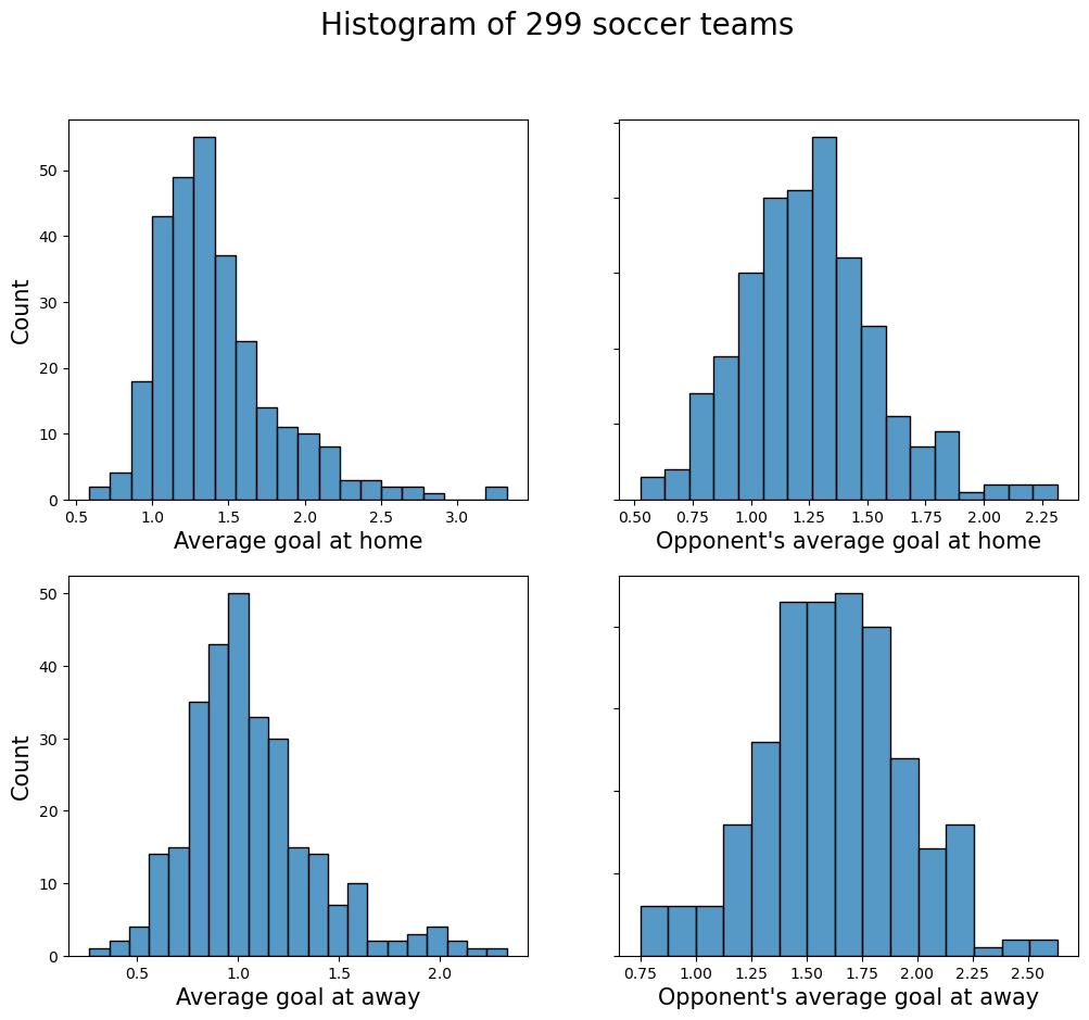
- It can be seen that the ability to score goals or block goals in home/away matches is very different for each team.
-
These differences will affect home and away win rates for each team.
- Let’s compare the best and worst 10% teams with the win rate at home.
fig, axes = plt.subplots(1, 2, figsize = (12, 5))

sns.boxplot(goal_match_result_info, x = "home_avg_goal", y = "home_win_class", ax = axes[0])
sns.boxplot(goal_match_result_info, x = "home_opponent_avg_goal", y = "home_win_class", ax = axes[1])

axes[0].set_ylabel("Home win class", fontsize = 15)
axes[0].set_xlabel("Average goal at home", fontsize = 15)

axes[1].set_ylabel("")
axes[1].set_xlabel("Opponent's average goal at home", fontsize = 15)
axes[1].yaxis.set_tick_params(labelleft = False)

plt.tight_layout()
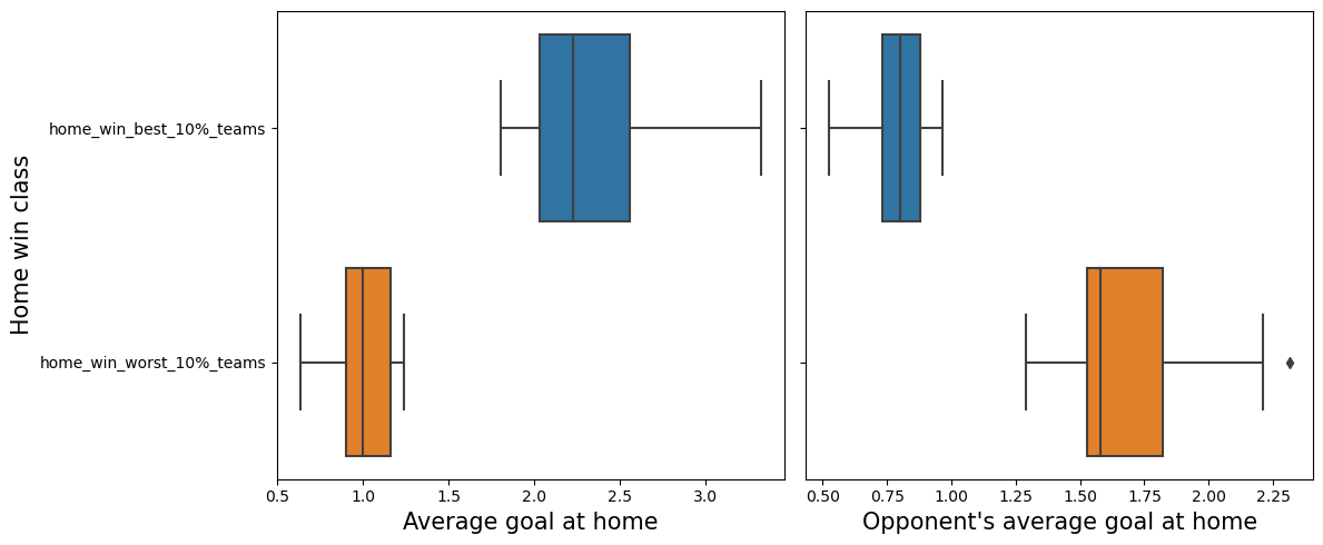
- Teams in the best 10% of home win percentage score an average of 1.2 more goals at home than teams in the worst 10%.
- For the best 10% teams with high win percentage at home, the average number of goals scored by the opposing team is around 0.8, very low compared to 1.6 from the worst 10% teams.
goal_match_result_info
| team_api_id | team_long_name | home_avg_goal | home_opponent_avg_goal | away_avg_goal | away_opponent_avg_goal | win_at_home | draw_at_home | lose_at_home | win_at_away | draw_at_away | lose_at_away | home_win_class | away_win_class | |
|---|---|---|---|---|---|---|---|---|---|---|---|---|---|---|
| 0 | 9930 | FC Aarau | 1.236111 | 1.652778 | 0.888889 | 2.152778 | 0.347222 | 0.166667 | 0.486111 | 0.138889 | 0.305556 | 0.555556 | NaN | NaN |
| 1 | 8485 | Aberdeen | 1.223684 | 0.967105 | 1.177632 | 1.381579 | 0.440789 | 0.250000 | 0.309211 | 0.348684 | 0.243421 | 0.407895 | NaN | NaN |
| 2 | 8576 | AC Ajaccio | 1.122807 | 1.350877 | 0.912281 | 1.877193 | 0.280702 | 0.333333 | 0.385965 | 0.105263 | 0.368421 | 0.526316 | NaN | away_win_worst_10%_teams |
| 3 | 8564 | Milan | 1.794702 | 0.847682 | 1.480263 | 1.210526 | 0.609272 | 0.225166 | 0.165563 | 0.407895 | 0.296053 | 0.296053 | NaN | NaN |
| 4 | 10215 | Académica de Coimbra | 1.096774 | 1.258065 | 0.838710 | 1.532258 | 0.282258 | 0.387097 | 0.330645 | 0.169355 | 0.274194 | 0.556452 | NaN | NaN |
| ... | ... | ... | ... | ... | ... | ... | ... | ... | ... | ... | ... | ... | ... | ... |
| 283 | 10192 | BSC Young Boys | 2.230769 | 1.160839 | 1.468531 | 1.447552 | 0.594406 | 0.237762 | 0.167832 | 0.398601 | 0.244755 | 0.356643 | NaN | NaN |
| 284 | 8021 | Zagłębie Lubin | 1.288889 | 1.200000 | 1.011111 | 1.377778 | 0.388889 | 0.300000 | 0.311111 | 0.266667 | 0.266667 | 0.466667 | NaN | NaN |
| 285 | 8394 | Real Zaragoza | 1.250000 | 1.328947 | 0.842105 | 1.828947 | 0.381579 | 0.223684 | 0.394737 | 0.184211 | 0.223684 | 0.592105 | NaN | NaN |
| 286 | 8027 | Zawisza Bydgoszcz | 1.433333 | 1.266667 | 1.066667 | 1.700000 | 0.433333 | 0.166667 | 0.400000 | 0.200000 | 0.300000 | 0.500000 | NaN | NaN |
| 287 | 10000 | SV Zulte-Waregem | 1.660377 | 1.273585 | 1.226415 | 1.367925 | 0.424528 | 0.301887 | 0.273585 | 0.311321 | 0.283019 | 0.405660 | NaN | NaN |
288 rows × 14 columns
fig, axes = plt.subplots(1, 2, figsize = (12, 5))

sns.boxplot(goal_match_result_info, x = "away_avg_goal", y = "away_win_class", ax = axes[0])
sns.boxplot(goal_match_result_info, x = "away_opponent_avg_goal", y = "away_win_class", ax = axes[1])

axes[0].set_ylabel("Away win class", fontsize = 15)
axes[0].set_xlabel("Average goal at away", fontsize = 15)

axes[1].set_ylabel("")
axes[1].set_xlabel("Opponent's average goal at away", fontsize = 15)
axes[1].yaxis.set_tick_params(labelleft = False)
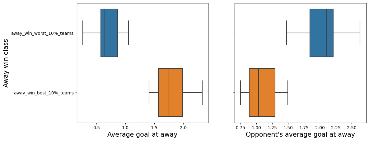
- Teams in the best 10% of away win percentage score an average of 1.2 more goals at away than teams in the worst 10%.
- For the best 10% teams with high win percentage at away, the average number of goals scored by the opposing team is around 1, very low compared to 2.2 from the worst 10% teams.
$\color{magenta} \quad \rightarrow$ So, let's create a variable for each team that indicates how well they score goals when home, how well they block goals when home, how well they score goals when away, and how well they block goals when away:
$\quad \quad$ - Each team’s last 1 / 3 / 5 / 10 / 20 / 30 / 60 / 90 matches
$\quad \quad \quad \quad$ - average goal at home
$\ \quad \quad \quad \quad$ - average opponent’s goal at home
$\ \quad \quad \quad \quad$ - average goal at away
$\ \quad \quad \quad \quad$ - average opponent’s goal at away
</font>
home_goal_info = df_match_basic[["home_team_api_id", "match_date", "season", "home_team_goal", "away_team_goal"]].sort_values(["home_team_api_id", "match_date"])
for i in [1, 3, 5, 10, 20, 30, 60, 90]:
    home_goal_info[f"home_team_avg_goal_at_home_last_{i}_matches"] = home_goal_info.groupby('home_team_api_id')['home_team_goal'].shift(1).rolling(i).mean()
    home_goal_info[f"home_team_avg_oppnt_goal_at_home_last_{i}_matches"] = home_goal_info.groupby('home_team_api_id')['away_team_goal'].shift(1).rolling(i).mean()
away_goal_info = df_match_basic[["away_team_api_id", "match_date", "season", "home_team_goal", "away_team_goal"]].sort_values(["away_team_api_id", "match_date"])
for i in [1, 3, 5, 10, 20, 30, 60, 90]:
    away_goal_info[f"away_team_avg_goal_at_away_last_{i}_matches"] = away_goal_info.groupby('away_team_api_id')['away_team_goal'].shift(1).rolling(i).mean()
    away_goal_info[f"away_team_avg_oppnt_goal_at_away_last_{i}_matches"] = away_goal_info.groupby('away_team_api_id')['home_team_goal'].shift(1).rolling(i).mean()
df_team_win_goal_rolling_features = df_match_basic[["match_api_id", "match_date", "home_team_api_id", "away_team_api_id"]]
df_team_win_goal_rolling_features = df_team_win_goal_rolling_features.merge(home_goal_info.drop(["season", "home_team_goal", "away_team_goal"], axis = 1), how = "left", on = ["match_date", "home_team_api_id"]) \
                                                                     .merge(away_goal_info.drop(["season", "home_team_goal", "away_team_goal"], axis = 1), how = "left", on = ["match_date", "away_team_api_id"])

df_team_win_goal_rolling_features
| match_api_id | match_date | home_team_api_id | away_team_api_id | home_team_avg_goal_at_home_last_1_matches | home_team_avg_oppnt_goal_at_home_last_1_matches | home_team_avg_goal_at_home_last_3_matches | home_team_avg_oppnt_goal_at_home_last_3_matches | home_team_avg_goal_at_home_last_5_matches | home_team_avg_oppnt_goal_at_home_last_5_matches | home_team_avg_goal_at_home_last_10_matches | home_team_avg_oppnt_goal_at_home_last_10_matches | home_team_avg_goal_at_home_last_20_matches | home_team_avg_oppnt_goal_at_home_last_20_matches | home_team_avg_goal_at_home_last_30_matches | home_team_avg_oppnt_goal_at_home_last_30_matches | home_team_avg_goal_at_home_last_60_matches | home_team_avg_oppnt_goal_at_home_last_60_matches | home_team_avg_goal_at_home_last_90_matches | home_team_avg_oppnt_goal_at_home_last_90_matches | away_team_avg_goal_at_away_last_1_matches | away_team_avg_oppnt_goal_at_away_last_1_matches | away_team_avg_goal_at_away_last_3_matches | away_team_avg_oppnt_goal_at_away_last_3_matches | away_team_avg_goal_at_away_last_5_matches | away_team_avg_oppnt_goal_at_away_last_5_matches | away_team_avg_goal_at_away_last_10_matches | away_team_avg_oppnt_goal_at_away_last_10_matches | away_team_avg_goal_at_away_last_20_matches | away_team_avg_oppnt_goal_at_away_last_20_matches | away_team_avg_goal_at_away_last_30_matches | away_team_avg_oppnt_goal_at_away_last_30_matches | away_team_avg_goal_at_away_last_60_matches | away_team_avg_oppnt_goal_at_away_last_60_matches | away_team_avg_goal_at_away_last_90_matches | away_team_avg_oppnt_goal_at_away_last_90_matches | |
|---|---|---|---|---|---|---|---|---|---|---|---|---|---|---|---|---|---|---|---|---|---|---|---|---|---|---|---|---|---|---|---|---|---|---|---|---|
| 0 | 492473 | 2008-08-17 | 9987 | 9993 | NaN | NaN | NaN | NaN | NaN | NaN | NaN | NaN | NaN | NaN | NaN | NaN | NaN | NaN | NaN | NaN | NaN | NaN | NaN | NaN | NaN | NaN | NaN | NaN | NaN | NaN | NaN | NaN | NaN | NaN | NaN | NaN |
| 1 | 492474 | 2008-08-16 | 10000 | 9994 | NaN | NaN | NaN | NaN | NaN | NaN | NaN | NaN | NaN | NaN | NaN | NaN | NaN | NaN | NaN | NaN | NaN | NaN | NaN | NaN | NaN | NaN | NaN | NaN | NaN | NaN | NaN | NaN | NaN | NaN | NaN | NaN |
| 2 | 492475 | 2008-08-16 | 9984 | 8635 | NaN | NaN | NaN | NaN | NaN | NaN | NaN | NaN | NaN | NaN | NaN | NaN | NaN | NaN | NaN | NaN | NaN | NaN | NaN | NaN | NaN | NaN | NaN | NaN | NaN | NaN | NaN | NaN | NaN | NaN | NaN | NaN |
| 3 | 492476 | 2008-08-17 | 9991 | 9998 | NaN | NaN | NaN | NaN | NaN | NaN | NaN | NaN | NaN | NaN | NaN | NaN | NaN | NaN | NaN | NaN | NaN | NaN | NaN | NaN | NaN | NaN | NaN | NaN | NaN | NaN | NaN | NaN | NaN | NaN | NaN | NaN |
| 4 | 492477 | 2008-08-16 | 7947 | 9985 | NaN | NaN | NaN | NaN | NaN | NaN | NaN | NaN | NaN | NaN | NaN | NaN | NaN | NaN | NaN | NaN | NaN | NaN | NaN | NaN | NaN | NaN | NaN | NaN | NaN | NaN | NaN | NaN | NaN | NaN | NaN | NaN |
| ... | ... | ... | ... | ... | ... | ... | ... | ... | ... | ... | ... | ... | ... | ... | ... | ... | ... | ... | ... | ... | ... | ... | ... | ... | ... | ... | ... | ... | ... | ... | ... | ... | ... | ... | ... | ... |
| 25974 | 1992091 | 2015-09-22 | 10190 | 10191 | 0.0 | 2.0 | 0.333333 | 1.666667 | 1.6 | 1.2 | 1.6 | 1.3 | 1.55 | 1.30 | 1.500000 | 1.333333 | 1.533333 | 1.133333 | 1.400000 | 1.311111 | 3.0 | 3.0 | 1.666667 | 3.000000 | 2.0 | 2.8 | 1.1 | 2.3 | 0.85 | 1.60 | 1.166667 | 1.600000 | 1.033333 | 1.500000 | 0.977778 | 1.377778 |
| 25975 | 1992092 | 2015-09-23 | 9824 | 10199 | 1.0 | 0.0 | 1.666667 | 1.333333 | 1.4 | 1.4 | 1.1 | 1.6 | 0.95 | 1.55 | 1.133333 | 1.866667 | NaN | NaN | NaN | NaN | 1.0 | 0.0 | 2.333333 | 0.666667 | 1.8 | 0.6 | 2.0 | 0.7 | 1.80 | 1.25 | 1.566667 | 1.533333 | 1.450000 | 1.633333 | 1.377778 | 1.588889 |
| 25976 | 1992093 | 2015-09-23 | 9956 | 10179 | 3.0 | 2.0 | 3.666667 | 2.000000 | 2.6 | 1.2 | 2.0 | 1.0 | 1.70 | 1.25 | 1.900000 | 1.333333 | 1.616667 | 1.133333 | 1.488889 | 1.222222 | 2.0 | 0.0 | 1.000000 | 1.333333 | 1.0 | 1.8 | 0.9 | 1.1 | 0.90 | 1.35 | 0.800000 | 1.366667 | 0.816667 | 1.550000 | 0.966667 | 1.355556 |
| 25977 | 1992094 | 2015-09-22 | 7896 | 10243 | 0.0 | 1.0 | 0.666667 | 1.333333 | NaN | NaN | NaN | NaN | NaN | NaN | NaN | NaN | NaN | NaN | NaN | NaN | 1.0 | 3.0 | 1.333333 | 2.000000 | 1.4 | 1.6 | 1.2 | 1.9 | 1.60 | 1.45 | 1.566667 | 1.500000 | 1.583333 | 1.500000 | 1.566667 | 1.455556 |
| 25978 | 1992095 | 2015-09-23 | 10192 | 9931 | 4.0 | 0.0 | 2.333333 | 0.666667 | 2.0 | 0.8 | 2.2 | 0.8 | 2.40 | 1.10 | 2.166667 | 1.266667 | 2.016667 | 1.166667 | 2.011111 | 1.222222 | 3.0 | 1.0 | 3.000000 | 1.333333 | 2.4 | 1.6 | 2.4 | 1.3 | 2.40 | 1.45 | 2.200000 | 1.266667 | 1.883333 | 1.166667 | 1.877778 | 1.188889 |
25979 rows × 36 columns
- Also let's use the each team's win or lose percentage at home and away for recent 1 / 3 / 5 / 10 / 20 / 30 / 60 / 90 matches.
home_win_info = df_match_basic[["home_team_api_id", "match_date", "match_result"]].sort_values(["home_team_api_id", "match_date"])
home_win_info.loc[home_win_info.match_result == "home_win", "is_win"] = 1
home_win_info.loc[home_win_info.match_result != "home_win", "is_win"] = 0

home_win_info.loc[home_win_info.match_result == "away_win", "is_lose"] = 1
home_win_info.loc[home_win_info.match_result != "away_win", "is_lose"] = 0
for i in [1, 3, 5, 10, 20, 30, 60, 90]:
    home_win_info[f"home_team_home_win_percentage_last_{i}_matches"] = home_win_info.groupby('home_team_api_id')['is_win'].shift(1).rolling(i).mean()
    home_win_info[f"home_team_home_lose_percentage_last_{i}_matches"] = home_win_info.groupby('home_team_api_id')['is_lose'].shift(1).rolling(i).mean()
away_win_info = df_match_basic[["away_team_api_id", "match_date", "match_result"]].sort_values(["away_team_api_id", "match_date"])
away_win_info.loc[away_win_info.match_result == "away_win", "is_win"] = 1
away_win_info.loc[away_win_info.match_result != "away_win", "is_win"] = 0

away_win_info.loc[away_win_info.match_result == "home_win", "is_lose"] = 1
away_win_info.loc[away_win_info.match_result != "home_win", "is_lose"] = 0
for i in [1, 3, 5, 10, 20, 30, 60, 90]:
    away_win_info[f"away_team_away_win_percentage_last_{i}_matches"] = away_win_info.groupby('away_team_api_id')['is_win'].shift(1).rolling(i).mean()
    away_win_info[f"away_team_away_lose_percentage_last_{i}_matches"] = away_win_info.groupby('away_team_api_id')['is_lose'].shift(1).rolling(i).mean()
df_team_win_goal_rolling_features = df_team_win_goal_rolling_features.merge(home_win_info.drop(["match_result", "is_win", "is_lose"], axis = 1), how = "left", on = ["match_date", "home_team_api_id"]) \
                                                                     .merge(away_win_info.drop(["match_result", "is_win", "is_lose"], axis = 1), how = "left", on = ["match_date", "away_team_api_id"]) \
                                                                     .drop(["match_date", "home_team_api_id", "away_team_api_id"], axis = 1)
df_team_win_goal_rolling_features
| match_api_id | home_team_avg_goal_at_home_last_1_matches | home_team_avg_oppnt_goal_at_home_last_1_matches | home_team_avg_goal_at_home_last_3_matches | home_team_avg_oppnt_goal_at_home_last_3_matches | home_team_avg_goal_at_home_last_5_matches | home_team_avg_oppnt_goal_at_home_last_5_matches | home_team_avg_goal_at_home_last_10_matches | home_team_avg_oppnt_goal_at_home_last_10_matches | home_team_avg_goal_at_home_last_20_matches | home_team_avg_oppnt_goal_at_home_last_20_matches | home_team_avg_goal_at_home_last_30_matches | home_team_avg_oppnt_goal_at_home_last_30_matches | home_team_avg_goal_at_home_last_60_matches | home_team_avg_oppnt_goal_at_home_last_60_matches | home_team_avg_goal_at_home_last_90_matches | home_team_avg_oppnt_goal_at_home_last_90_matches | away_team_avg_goal_at_away_last_1_matches | away_team_avg_oppnt_goal_at_away_last_1_matches | away_team_avg_goal_at_away_last_3_matches | away_team_avg_oppnt_goal_at_away_last_3_matches | away_team_avg_goal_at_away_last_5_matches | away_team_avg_oppnt_goal_at_away_last_5_matches | away_team_avg_goal_at_away_last_10_matches | away_team_avg_oppnt_goal_at_away_last_10_matches | away_team_avg_goal_at_away_last_20_matches | away_team_avg_oppnt_goal_at_away_last_20_matches | away_team_avg_goal_at_away_last_30_matches | away_team_avg_oppnt_goal_at_away_last_30_matches | away_team_avg_goal_at_away_last_60_matches | away_team_avg_oppnt_goal_at_away_last_60_matches | away_team_avg_goal_at_away_last_90_matches | away_team_avg_oppnt_goal_at_away_last_90_matches | home_team_home_win_percentage_last_1_matches | home_team_home_lose_percentage_last_1_matches | home_team_home_win_percentage_last_3_matches | home_team_home_lose_percentage_last_3_matches | home_team_home_win_percentage_last_5_matches | home_team_home_lose_percentage_last_5_matches | home_team_home_win_percentage_last_10_matches | home_team_home_lose_percentage_last_10_matches | home_team_home_win_percentage_last_20_matches | home_team_home_lose_percentage_last_20_matches | home_team_home_win_percentage_last_30_matches | home_team_home_lose_percentage_last_30_matches | home_team_home_win_percentage_last_60_matches | home_team_home_lose_percentage_last_60_matches | home_team_home_win_percentage_last_90_matches | home_team_home_lose_percentage_last_90_matches | away_team_away_win_percentage_last_1_matches | away_team_away_lose_percentage_last_1_matches | away_team_away_win_percentage_last_3_matches | away_team_away_lose_percentage_last_3_matches | away_team_away_win_percentage_last_5_matches | away_team_away_lose_percentage_last_5_matches | away_team_away_win_percentage_last_10_matches | away_team_away_lose_percentage_last_10_matches | away_team_away_win_percentage_last_20_matches | away_team_away_lose_percentage_last_20_matches | away_team_away_win_percentage_last_30_matches | away_team_away_lose_percentage_last_30_matches | away_team_away_win_percentage_last_60_matches | away_team_away_lose_percentage_last_60_matches | away_team_away_win_percentage_last_90_matches | away_team_away_lose_percentage_last_90_matches | |
|---|---|---|---|---|---|---|---|---|---|---|---|---|---|---|---|---|---|---|---|---|---|---|---|---|---|---|---|---|---|---|---|---|---|---|---|---|---|---|---|---|---|---|---|---|---|---|---|---|---|---|---|---|---|---|---|---|---|---|---|---|---|---|---|---|---|
| 0 | 492473 | NaN | NaN | NaN | NaN | NaN | NaN | NaN | NaN | NaN | NaN | NaN | NaN | NaN | NaN | NaN | NaN | NaN | NaN | NaN | NaN | NaN | NaN | NaN | NaN | NaN | NaN | NaN | NaN | NaN | NaN | NaN | NaN | NaN | NaN | NaN | NaN | NaN | NaN | NaN | NaN | NaN | NaN | NaN | NaN | NaN | NaN | NaN | NaN | NaN | NaN | NaN | NaN | NaN | NaN | NaN | NaN | NaN | NaN | NaN | NaN | NaN | NaN | NaN | NaN |
| 1 | 492474 | NaN | NaN | NaN | NaN | NaN | NaN | NaN | NaN | NaN | NaN | NaN | NaN | NaN | NaN | NaN | NaN | NaN | NaN | NaN | NaN | NaN | NaN | NaN | NaN | NaN | NaN | NaN | NaN | NaN | NaN | NaN | NaN | NaN | NaN | NaN | NaN | NaN | NaN | NaN | NaN | NaN | NaN | NaN | NaN | NaN | NaN | NaN | NaN | NaN | NaN | NaN | NaN | NaN | NaN | NaN | NaN | NaN | NaN | NaN | NaN | NaN | NaN | NaN | NaN |
| 2 | 492475 | NaN | NaN | NaN | NaN | NaN | NaN | NaN | NaN | NaN | NaN | NaN | NaN | NaN | NaN | NaN | NaN | NaN | NaN | NaN | NaN | NaN | NaN | NaN | NaN | NaN | NaN | NaN | NaN | NaN | NaN | NaN | NaN | NaN | NaN | NaN | NaN | NaN | NaN | NaN | NaN | NaN | NaN | NaN | NaN | NaN | NaN | NaN | NaN | NaN | NaN | NaN | NaN | NaN | NaN | NaN | NaN | NaN | NaN | NaN | NaN | NaN | NaN | NaN | NaN |
| 3 | 492476 | NaN | NaN | NaN | NaN | NaN | NaN | NaN | NaN | NaN | NaN | NaN | NaN | NaN | NaN | NaN | NaN | NaN | NaN | NaN | NaN | NaN | NaN | NaN | NaN | NaN | NaN | NaN | NaN | NaN | NaN | NaN | NaN | NaN | NaN | NaN | NaN | NaN | NaN | NaN | NaN | NaN | NaN | NaN | NaN | NaN | NaN | NaN | NaN | NaN | NaN | NaN | NaN | NaN | NaN | NaN | NaN | NaN | NaN | NaN | NaN | NaN | NaN | NaN | NaN |
| 4 | 492477 | NaN | NaN | NaN | NaN | NaN | NaN | NaN | NaN | NaN | NaN | NaN | NaN | NaN | NaN | NaN | NaN | NaN | NaN | NaN | NaN | NaN | NaN | NaN | NaN | NaN | NaN | NaN | NaN | NaN | NaN | NaN | NaN | NaN | NaN | NaN | NaN | NaN | NaN | NaN | NaN | NaN | NaN | NaN | NaN | NaN | NaN | NaN | NaN | NaN | NaN | NaN | NaN | NaN | NaN | NaN | NaN | NaN | NaN | NaN | NaN | NaN | NaN | NaN | NaN |
| ... | ... | ... | ... | ... | ... | ... | ... | ... | ... | ... | ... | ... | ... | ... | ... | ... | ... | ... | ... | ... | ... | ... | ... | ... | ... | ... | ... | ... | ... | ... | ... | ... | ... | ... | ... | ... | ... | ... | ... | ... | ... | ... | ... | ... | ... | ... | ... | ... | ... | ... | ... | ... | ... | ... | ... | ... | ... | ... | ... | ... | ... | ... | ... | ... | ... |
| 25974 | 1992091 | 0.0 | 2.0 | 0.333333 | 1.666667 | 1.6 | 1.2 | 1.6 | 1.3 | 1.55 | 1.30 | 1.500000 | 1.333333 | 1.533333 | 1.133333 | 1.400000 | 1.311111 | 3.0 | 3.0 | 1.666667 | 3.000000 | 2.0 | 2.8 | 1.1 | 2.3 | 0.85 | 1.60 | 1.166667 | 1.600000 | 1.033333 | 1.500000 | 0.977778 | 1.377778 | 0.0 | 1.0 | 0.000000 | 0.666667 | 0.4 | 0.4 | 0.4 | 0.4 | 0.40 | 0.30 | 0.4 | 0.266667 | 0.450000 | 0.233333 | 0.388889 | 0.333333 | 0.0 | 0.0 | 0.000000 | 0.666667 | 0.2 | 0.6 | 0.1 | 0.6 | 0.15 | 0.45 | 0.233333 | 0.466667 | 0.233333 | 0.516667 | 0.255556 | 0.477778 |
| 25975 | 1992092 | 1.0 | 0.0 | 1.666667 | 1.333333 | 1.4 | 1.4 | 1.1 | 1.6 | 0.95 | 1.55 | 1.133333 | 1.866667 | NaN | NaN | NaN | NaN | 1.0 | 0.0 | 2.333333 | 0.666667 | 1.8 | 0.6 | 2.0 | 0.7 | 1.80 | 1.25 | 1.566667 | 1.533333 | 1.450000 | 1.633333 | 1.377778 | 1.588889 | 1.0 | 0.0 | 0.333333 | 0.000000 | 0.2 | 0.2 | 0.2 | 0.5 | 0.20 | 0.45 | 0.2 | 0.500000 | NaN | NaN | NaN | NaN | 1.0 | 0.0 | 1.000000 | 0.000000 | 0.8 | 0.0 | 0.8 | 0.1 | 0.50 | 0.30 | 0.400000 | 0.433333 | 0.350000 | 0.450000 | 0.311111 | 0.455556 |
| 25976 | 1992093 | 3.0 | 2.0 | 3.666667 | 2.000000 | 2.6 | 1.2 | 2.0 | 1.0 | 1.70 | 1.25 | 1.900000 | 1.333333 | 1.616667 | 1.133333 | 1.488889 | 1.222222 | 2.0 | 0.0 | 1.000000 | 1.333333 | 1.0 | 1.8 | 0.9 | 1.1 | 0.90 | 1.35 | 0.800000 | 1.366667 | 0.816667 | 1.550000 | 0.966667 | 1.355556 | 1.0 | 0.0 | 0.666667 | 0.333333 | 0.6 | 0.2 | 0.5 | 0.1 | 0.45 | 0.30 | 0.5 | 0.300000 | 0.500000 | 0.283333 | 0.466667 | 0.333333 | 1.0 | 0.0 | 0.333333 | 0.333333 | 0.2 | 0.4 | 0.4 | 0.3 | 0.25 | 0.45 | 0.233333 | 0.500000 | 0.233333 | 0.550000 | 0.266667 | 0.466667 |
| 25977 | 1992094 | 0.0 | 1.0 | 0.666667 | 1.333333 | NaN | NaN | NaN | NaN | NaN | NaN | NaN | NaN | NaN | NaN | NaN | NaN | 1.0 | 3.0 | 1.333333 | 2.000000 | 1.4 | 1.6 | 1.2 | 1.9 | 1.60 | 1.45 | 1.566667 | 1.500000 | 1.583333 | 1.500000 | 1.566667 | 1.455556 | 0.0 | 1.0 | 0.333333 | 0.666667 | NaN | NaN | NaN | NaN | NaN | NaN | NaN | NaN | NaN | NaN | NaN | NaN | 0.0 | 1.0 | 0.333333 | 0.666667 | 0.4 | 0.4 | 0.3 | 0.4 | 0.45 | 0.30 | 0.466667 | 0.366667 | 0.450000 | 0.350000 | 0.455556 | 0.355556 |
| 25978 | 1992095 | 4.0 | 0.0 | 2.333333 | 0.666667 | 2.0 | 0.8 | 2.2 | 0.8 | 2.40 | 1.10 | 2.166667 | 1.266667 | 2.016667 | 1.166667 | 2.011111 | 1.222222 | 3.0 | 1.0 | 3.000000 | 1.333333 | 2.4 | 1.6 | 2.4 | 1.3 | 2.40 | 1.45 | 2.200000 | 1.266667 | 1.883333 | 1.166667 | 1.877778 | 1.188889 | 1.0 | 0.0 | 0.666667 | 0.333333 | 0.6 | 0.2 | 0.6 | 0.2 | 0.70 | 0.20 | 0.6 | 0.200000 | 0.566667 | 0.233333 | 0.522222 | 0.211111 | 1.0 | 0.0 | 1.000000 | 0.000000 | 0.6 | 0.2 | 0.7 | 0.1 | 0.70 | 0.20 | 0.666667 | 0.166667 | 0.533333 | 0.183333 | 0.511111 | 0.155556 |
25979 rows × 65 columns
- Save the table.
df_team_win_goal_rolling_features.to_csv("../data/df_team_win_goal_rolling_features.csv", index = False)
1.3. Elapsed time of goals
Q. Are there specific times when goals are scored most?
plt.figure(figsize = (20, 10))
sns.histplot(data = df_match_ingame_shot_goal, x = "elapsed")
plt.xlabel("Elapsed time of goals", fontsize = 20)
plt.ylabel("count", fontsize = 20)
plt.vlines(x = 45, ymin = 0, ymax = 3500, colors = "red", linewidth = 3)
plt.vlines(x = 90, ymin = 0, ymax = 3500, colors = "red", linewidth = 3)
plt.text(x = 33, y = 3550, s = "End of the first half", color = "red", fontsize = 15)
plt.text(x = 75, y = 3550, s = "End of the second half", color = "red", fontsize = 15)
plt.title("Histogram of the elapsed time of goals", fontsize = 25)
Text(0.5, 1.0, 'Histogram of the elapsed time of goals')
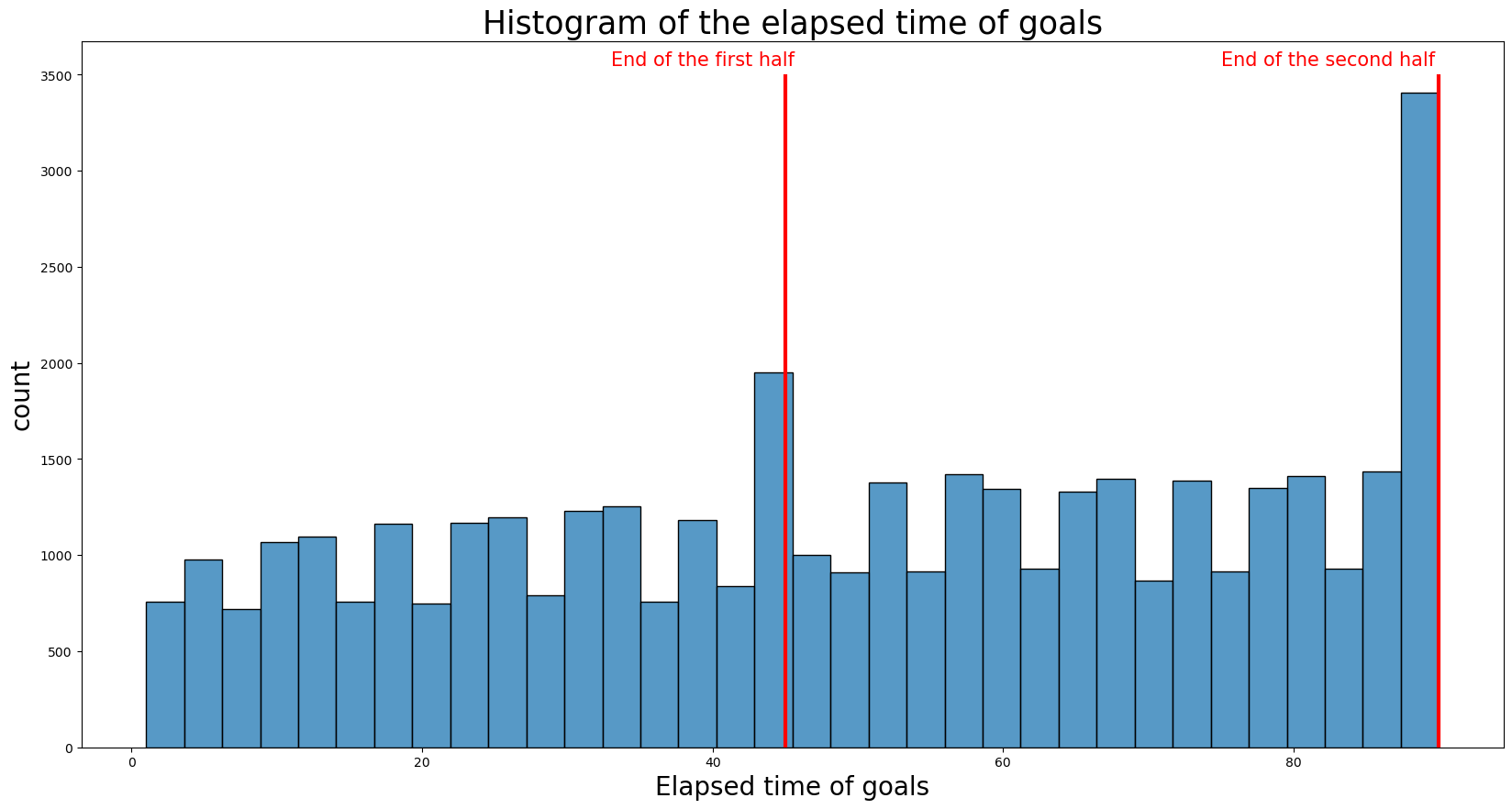
- Elapsed time of goals is almost uniformly distributed except for the right before the end of first and second half where a lot of goals are scored.
Q: Is there any difference in the distribution of the elapsed time of goals between winning and losing team ?
df_match_ingame_shot_goal
| match_api_id | event_id | elapsed | team_api_id | category | type | subtype | player1_api_id | player2_api_id | match_date | match_result | season | home_away | league_name | |
|---|---|---|---|---|---|---|---|---|---|---|---|---|---|---|
| 0 | 489042 | 378998 | 22 | 10261.0 | goal | n | header | 37799.0 | 38807.0 | 2008-08-17 | draw | 2008/2009 | away | England Premier League |
| 1 | 489042 | 379019 | 24 | 10260.0 | goal | n | shot | 24148.0 | 24154.0 | 2008-08-17 | draw | 2008/2009 | home | England Premier League |
| 2 | 489043 | 375546 | 4 | 9825.0 | goal | n | shot | 26181.0 | 39297.0 | 2008-08-16 | home_win | 2008/2009 | home | England Premier League |
| 3 | 489044 | 378041 | 83 | 8650.0 | goal | n | distance | 30853.0 | 30889.0 | 2008-08-16 | away_win | 2008/2009 | away | England Premier League |
| 4 | 489045 | 376060 | 4 | 8654.0 | goal | n | shot | 23139.0 | 36394.0 | 2008-08-16 | home_win | 2008/2009 | home | England Premier League |
| ... | ... | ... | ... | ... | ... | ... | ... | ... | ... | ... | ... | ... | ... | ... |
| 39975 | 1992228 | 5640015 | 71 | 10192.0 | goal | n | NaN | 37554.0 | NaN | 2016-05-25 | away_win | 2015/2016 | away | Switzerland Super League |
| 39976 | 1992229 | 5639993 | 58 | 9824.0 | goal | n | NaN | 493418.0 | NaN | 2016-05-25 | home_win | 2015/2016 | away | Switzerland Super League |
| 39977 | 1992229 | 5640008 | 67 | 10243.0 | goal | n | NaN | 197757.0 | NaN | 2016-05-25 | home_win | 2015/2016 | home | Switzerland Super League |
| 39978 | 1992229 | 5640010 | 69 | 10243.0 | goal | n | NaN | 198082.0 | NaN | 2016-05-25 | home_win | 2015/2016 | home | Switzerland Super League |
| 39979 | 1992229 | 5640020 | 76 | 10243.0 | goal | n | NaN | 121080.0 | NaN | 2016-05-25 | home_win | 2015/2016 | home | Switzerland Super League |
39980 rows × 14 columns
win_team = pd.concat([df_match_ingame_shot_goal[(df_match_ingame_shot_goal.match_result == "home_win") & (df_match_ingame_shot_goal.home_away == "home")],
                      df_match_ingame_shot_goal[(df_match_ingame_shot_goal.match_result == "away_win") & (df_match_ingame_shot_goal.home_away == "away")]])

lose_team = pd.concat([df_match_ingame_shot_goal[(df_match_ingame_shot_goal.match_result == "home_win") & (df_match_ingame_shot_goal.home_away == "away")],
                      df_match_ingame_shot_goal[(df_match_ingame_shot_goal.match_result == "away_win") & (df_match_ingame_shot_goal.home_away == "home")]])
win_team["win_lose"] = "win_team"
lose_team["win_lose"] = "lose_team"

elapsed_win_lose = pd.concat([win_team[["elapsed", "win_lose"]], lose_team[["elapsed", "win_lose"]]])
plt.figure(figsize = (20, 10))
sns.histplot(elapsed_win_lose, x = "elapsed", hue = "win_lose")
plt.xlabel("Elapsed time of goals", fontsize = 20)
plt.ylabel("count", fontsize = 20)
plt.vlines(x = 45, ymin = 0, ymax = 3500, colors = "red", linewidth = 3)
plt.vlines(x = 90, ymin = 0, ymax = 3500, colors = "red", linewidth = 3)
plt.text(x = 33, y = 3550, s = "End of the first half", color = "red", fontsize = 15)
plt.text(x = 75, y = 3550, s = "End of the second half", color = "red", fontsize = 15)
plt.title("Histogram of the elapsed time of goals", fontsize = 25)

top = mpatches.Patch(color = "skyblue", label = 'Winning team')
bottom = mpatches.Patch(color = "orange", label = 'Losing team')
plt.legend(handles=[top, bottom], loc = "upper left", fontsize = 15)
<matplotlib.legend.Legend at 0x7ff683f6e140>
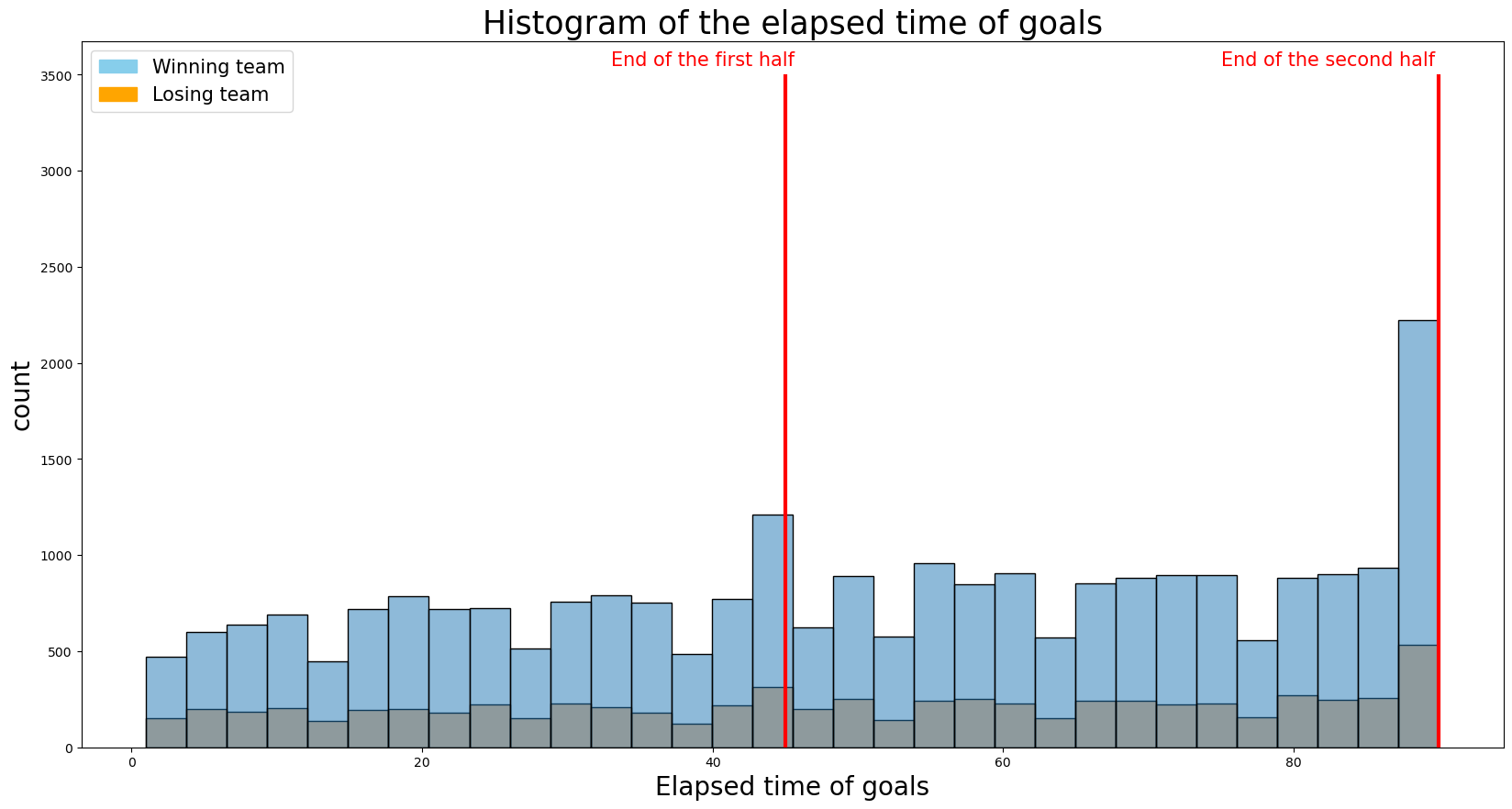
- The losing team scores fewer goals, but there is no difference in the overall shape of the distribution of elapsed time of goals between the winning and losing team.
Q: Is there any difference in the distribution of the elapsed time of goals between home and away team ?
plt.figure(figsize = (20, 10))
sns.histplot(df_match_ingame_shot_goal, x = "elapsed", hue = "home_away")
plt.xlabel("Elapsed time of goals", fontsize = 20)
plt.ylabel("count", fontsize = 20)
plt.vlines(x = 45, ymin = 0, ymax = 3500, colors = "red", linewidth = 3)
plt.vlines(x = 90, ymin = 0, ymax = 3500, colors = "red", linewidth = 3)
plt.text(x = 33, y = 3550, s = "End of the first half", color = "red", fontsize = 15)
plt.text(x = 75, y = 3550, s = "End of the second half", color = "red", fontsize = 15)
plt.title("Histogram of the elapsed time of goals", fontsize = 25)

top = mpatches.Patch(color = "orange", label = 'Home team')
bottom = mpatches.Patch(color = "skyblue", label = 'Away team')
plt.legend(handles=[top, bottom], loc = "upper left", fontsize = 15)
<matplotlib.legend.Legend at 0x7ff683f4a740>
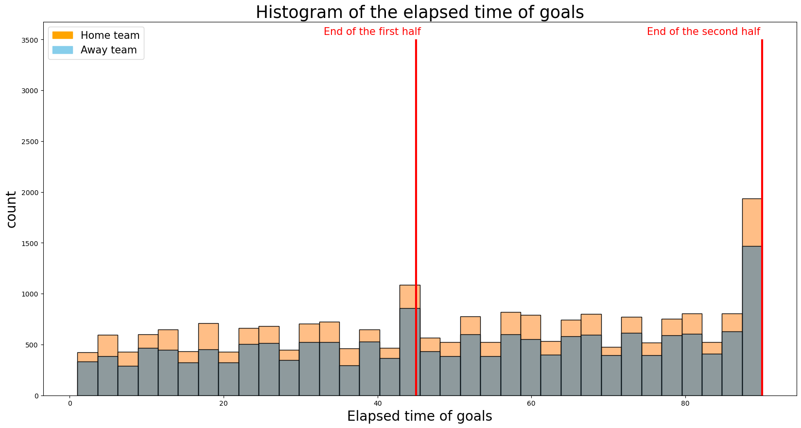
- The away team scores fewer goals, but there is no difference in the overall shape of the distribution of elapsed time of goals between the home and away team.
$\color{magenta} \quad \rightarrow$ The elapsed time of goals doesn't seem to make much of a difference between home & away teams or winning & losing teams. Therefore, we decided not to use it in modeling.
2. Shot
df_match_ingame_shot_shot = df_match_ingame_shot[df_match_ingame_shot.category == "shot"]
df_match_ingame_shot_shot
| match_api_id | event_id | elapsed | team_api_id | category | type | subtype | player1_api_id | player2_api_id | match_date | match_result | season | home_away | league_name | |
|---|---|---|---|---|---|---|---|---|---|---|---|---|---|---|
| 39980 | 489042 | 378828 | 3 | 10260.0 | shot | shoton | NaN | 24154.0 | NaN | 2008-08-17 | draw | 2008/2009 | home | England Premier League |
| 39981 | 489042 | 378866 | 7 | 10260.0 | shot | shoton | NaN | 24157.0 | NaN | 2008-08-17 | draw | 2008/2009 | home | England Premier League |
| 39982 | 489042 | 378922 | 14 | 10260.0 | shot | shoton | NaN | 30829.0 | NaN | 2008-08-17 | draw | 2008/2009 | home | England Premier League |
| 39983 | 489042 | 378923 | 14 | 10260.0 | shot | shoton | NaN | 30373.0 | NaN | 2008-08-17 | draw | 2008/2009 | home | England Premier League |
| 39984 | 489042 | 378951 | 17 | 10260.0 | shot | shoton | NaN | 30373.0 | NaN | 2008-08-17 | draw | 2008/2009 | home | England Premier League |
| ... | ... | ... | ... | ... | ... | ... | ... | ... | ... | ... | ... | ... | ... | ... |
| 229033 | 2030171 | 4940379 | 19 | 8370.0 | shot | shotoff | NaN | 36130.0 | NaN | 2015-10-23 | home_win | 2015/2016 | home | Spain LIGA BBVA |
| 229034 | 2030171 | 4940624 | 44 | 8370.0 | shot | shotoff | NaN | 34104.0 | NaN | 2015-10-23 | home_win | 2015/2016 | home | Spain LIGA BBVA |
| 229035 | 2030171 | 4940738 | 49 | 8558.0 | shot | shotoff | NaN | 107930.0 | NaN | 2015-10-23 | home_win | 2015/2016 | away | Spain LIGA BBVA |
| 229036 | 2030171 | 4940963 | 71 | 8370.0 | shot | shotoff | NaN | 210065.0 | NaN | 2015-10-23 | home_win | 2015/2016 | home | Spain LIGA BBVA |
| 229037 | 2030171 | 4941072 | 83 | 8558.0 | shot | shotoff | NaN | 629579.0 | NaN | 2015-10-23 | home_win | 2015/2016 | away | Spain LIGA BBVA |
189058 rows × 14 columns
df_match_ingame_shot_shot.type.value_counts()
shotoff    95303
shoton     93755
Name: type, dtype: int64
- There are two kinds of shot type:
- shoton: It means shot on target. Definition of the shot on target is as follow.
- Goes into the net regardless of intent.
- Is a clear attempt to score that would have gone into the net but for being saved by the goalkeeper or is stopped by a player who is the last line of defence with the goalkeeper having no chance of preventing the goal (last line block).
- shotoff: It means shot off target. Definition of the shot on target is as follow.
- Goes over or wide of the goal without making contact with another player.
- Would have gone over or wide of the goal but for being stopped by a goalkeeper’s save or by an outfield player.
- Directly hits the frame of the goal and a goal is not scored.
- shoton: It means shot on target. Definition of the shot on target is as follow.
sns.countplot(x = df_match_ingame_shot_shot.type)
<AxesSubplot:xlabel='type', ylabel='count'>
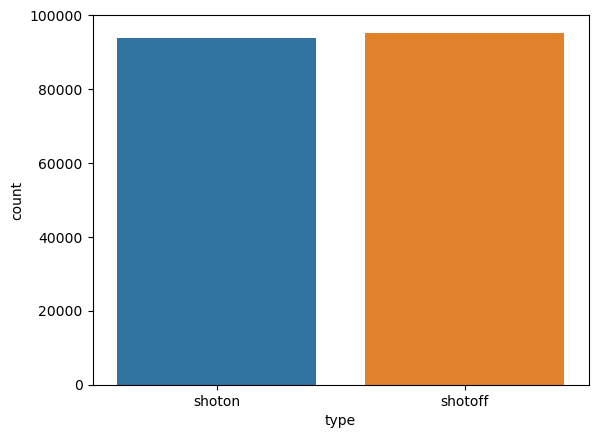
- The portion of the shot on target and the shot off target out of total shot are almost same.
Q. Are there any relationship between total number of shot, total number of shot on target, and total number of shot off target and number of goals.
goal_info = df_match_ingame_shot_goal.groupby(["match_api_id", "team_api_id"]).event_id.count().reset_index().rename(columns = {"event_id": "num_goals"})
shot_info = df_match_ingame_shot_shot.groupby(["match_api_id", "team_api_id"]).event_id.count().reset_index().rename(columns = {"event_id": "num_shots"})
shot_on_info = df_match_ingame_shot_shot[df_match_ingame_shot_shot.type == "shoton"].groupby(["match_api_id", "team_api_id"]).event_id.count().reset_index().rename(columns = {"event_id": "num_shots_on"})
shot_off_info = df_match_ingame_shot_shot[df_match_ingame_shot_shot.type == "shotoff"].groupby(["match_api_id", "team_api_id"]).event_id.count().reset_index().rename(columns = {"event_id": "num_shots_off"})
goal_shot_info = shot_info.merge(goal_info, how = "left", on = ["match_api_id", "team_api_id"]) \
                          .merge(shot_on_info, how = "left", on = ["match_api_id", "team_api_id"]) \
                          .merge(shot_off_info, how = "left", on = ["match_api_id", "team_api_id"]) \
                          [["match_api_id", "team_api_id", "num_shots_on", "num_shots_off", "num_shots", "num_goals"]] \
                          .fillna(0)
goal_shot_info[["num_shots_on", "num_shots_off", "num_shots", "num_goals"]].corr()
| num_shots_on | num_shots_off | num_shots | num_goals | |
|---|---|---|---|---|
| num_shots_on | 1.000000 | 0.328353 | 0.827919 | 0.105083 |
| num_shots_off | 0.328353 | 1.000000 | 0.801601 | 0.061156 |
| num_shots | 0.827919 | 0.801601 | 1.000000 | 0.102825 |
| num_goals | 0.105083 | 0.061156 | 0.102825 | 1.000000 |
- If we check the correlations, the number of shot on target and the number of shots have higher correlation with the number of goals than the number of shot off.
Q. Is there any difference in the distribution of number of shots between winning team and losing team ?
target_bool = ((df_match_ingame_shot_shot.match_result == "home_win") & (df_match_ingame_shot_shot.home_away == "home")) | ((df_match_ingame_shot_shot.match_result == "away_win") & (df_match_ingame_shot_shot.home_away == "away"))
win_shot_info = df_match_ingame_shot_shot[target_bool].groupby(["match_api_id", "team_api_id"]).count().event_id.reset_index().rename(columns = {"event_id": "values"})
win_shot_info["category"] = "shots"
win_shot_info["win_loss"] = "win"
target_bool = ((df_match_ingame_shot_shot.match_result == "home_win") & (df_match_ingame_shot_shot.home_away == "away")) | ((df_match_ingame_shot_shot.match_result == "away_win") & (df_match_ingame_shot_shot.home_away == "home"))
lose_shot_info = df_match_ingame_shot_shot[target_bool].groupby(["match_api_id", "team_api_id"]).count().event_id.reset_index().rename(columns = {"event_id": "values"})
lose_shot_info["category"] = "shots"
lose_shot_info["win_loss"] = "lose"
target_bool = ((df_match_ingame_shot_shot.match_result == "home_win") & (df_match_ingame_shot_shot.home_away == "home")) | ((df_match_ingame_shot_shot.match_result == "away_win") & (df_match_ingame_shot_shot.home_away == "away"))
shot_on_bool = df_match_ingame_shot_shot.type == "shoton"
win_shot_on_info = df_match_ingame_shot_shot[target_bool & shot_on_bool].groupby(["match_api_id", "team_api_id"]).count().event_id.reset_index().rename(columns = {"event_id": "values"})
win_shot_on_info["category"] = "shot_on"
win_shot_on_info["win_loss"] = "win"
target_bool = ((df_match_ingame_shot_shot.match_result == "home_win") & (df_match_ingame_shot_shot.home_away == "away")) | ((df_match_ingame_shot_shot.match_result == "away_win") & (df_match_ingame_shot_shot.home_away == "home"))
shot_on_bool = df_match_ingame_shot_shot.type == "shoton"
lose_shot_on_info = df_match_ingame_shot_shot[target_bool & shot_on_bool].groupby(["match_api_id", "team_api_id"]).count().event_id.reset_index().rename(columns = {"event_id": "values"})
lose_shot_on_info["category"] = "shot_on"
lose_shot_on_info["win_loss"] = "lose"
target_bool = ((df_match_ingame_shot_shot.match_result == "home_win") & (df_match_ingame_shot_shot.home_away == "home")) | ((df_match_ingame_shot_shot.match_result == "away_win") & (df_match_ingame_shot_shot.home_away == "away"))
shot_on_bool = df_match_ingame_shot_shot.type == "shotoff"
win_shot_off_info = df_match_ingame_shot_shot[target_bool & shot_on_bool].groupby(["match_api_id", "team_api_id"]).count().event_id.reset_index().rename(columns = {"event_id": "values"})
win_shot_off_info["category"] = "shot_off"
win_shot_off_info["win_loss"] = "win"
target_bool = ((df_match_ingame_shot_shot.match_result == "home_win") & (df_match_ingame_shot_shot.home_away == "away")) | ((df_match_ingame_shot_shot.match_result == "away_win") & (df_match_ingame_shot_shot.home_away == "home"))
shot_on_bool = df_match_ingame_shot_shot.type == "shotoff"
lose_shot_off_info = df_match_ingame_shot_shot[target_bool & shot_on_bool].groupby(["match_api_id", "team_api_id"]).count().event_id.reset_index().rename(columns = {"event_id": "values"})
lose_shot_off_info["category"] = "shot_off"
lose_shot_off_info["win_loss"] = "lose"
win_lose_shot_info = pd.concat([win_shot_info, lose_shot_info, win_shot_on_info, lose_shot_on_info, win_shot_off_info, lose_shot_off_info])
fig, axes = plt.subplots(1, 3, figsize = (18, 5))

sns.histplot(data = win_lose_shot_info[win_lose_shot_info.category == "shots"], x = "values", hue = "win_loss", ax = axes[0])
axes[0].set_xlabel("Total number of shots", fontsize = 15)
axes[0].set_ylabel("Count", fontsize = 15)

sns.histplot(data = win_lose_shot_info[win_lose_shot_info.category == "shot_on"], x = "values", hue = "win_loss", ax = axes[1])
axes[1].set_xlabel("Total number of shots on target", fontsize = 15)
axes[1].set_ylabel("Count", fontsize = 15)

sns.histplot(data = win_lose_shot_info[win_lose_shot_info.category == "shot_off"], x = "values", hue = "win_loss", ax = axes[2])
axes[2].set_xlabel("Total number of shots off target", fontsize = 15)
axes[2].set_ylabel("Count", fontsize = 15)
Text(0, 0.5, 'Count')
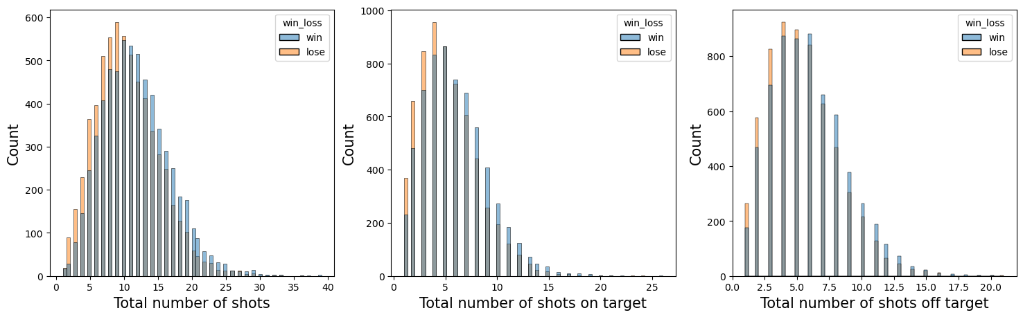
- The shape of the distribution of the winning team and the losing team is the same, but the distribution of the winning team is shifted slightly to the right.
- It can be seen that the winning teams took slightly more shots overall.
Q. Is there any difference of shot on target ratio(the number of shots on target / the number of shots) between winnint team and losing team ?
win_lose_shot_info = win_shot_info[["match_api_id", "values"]].rename(columns = {"values": "win_num_shots"}).merge(lose_shot_info[["match_api_id", "values"]].rename(columns = {"values": "lose_num_shots"}), how = "left", on = "match_api_id") \
                                                                                                            .merge(win_shot_on_info[["match_api_id", "values"]].rename(columns = {"values": "win_num_shot_on"}), how = "left", on = "match_api_id") \
                                                                                                            .merge(lose_shot_on_info[["match_api_id", "values"]].rename(columns = {"values": "lose_num_shot_on"}), how = "left", on = "match_api_id") \
                                                                                                            .merge(win_shot_off_info[["match_api_id", "values"]].rename(columns = {"values": "win_num_shot_off"}), how = "left", on = "match_api_id") \
                                                                                                            .merge(lose_shot_off_info[["match_api_id", "values"]].rename(columns = {"values": "lose_num_shot_off"}), how = "left", on = "match_api_id")
win_lose_shot_info["win_shot_ratio"] = win_lose_shot_info.win_num_shot_on / win_lose_shot_info.win_num_shots
win_lose_shot_info["lose_shot_ratio"] = win_lose_shot_info.lose_num_shot_on / win_lose_shot_info.lose_num_shots
win_lose_shot_info["shot_on_target_ratio_difference"] = win_lose_shot_info.win_shot_ratio - win_lose_shot_info.lose_shot_ratio
my_histogram(win_lose_shot_info, "shot_on_target_ratio_difference")
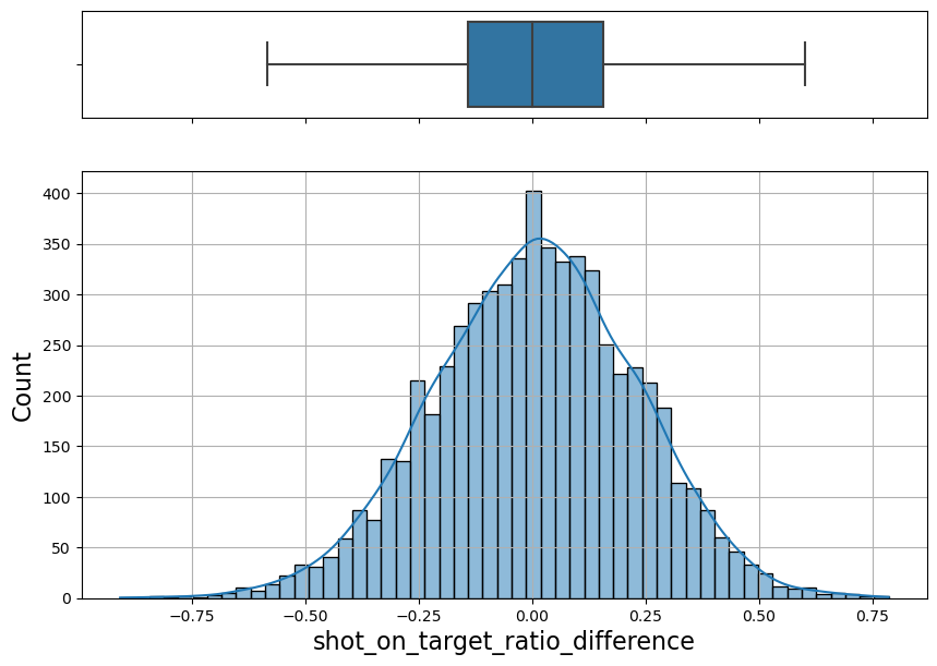
- Above plot shows the histogram of the shot on target ratio difference between the winning team and the losing team.
- There are also half of the matches where the losing team had the higher shot on target ratio.
- Since the distribution is symmetric, it is difficult to say that the winning team had the particularly higher shot on target ratio than that of the losing team.
Q. Is there any difference in the distribution of number of shots between home team and away team ?
home_shot_info = df_match_ingame_shot_shot[df_match_ingame_shot_shot.home_away == "home"].groupby(["match_api_id", "team_api_id"]).count().event_id.reset_index().rename(columns = {"event_id": "home_num_shots"}).drop("team_api_id", axis = 1)
away_shot_info = df_match_ingame_shot_shot[df_match_ingame_shot_shot.home_away == "away"].groupby(["match_api_id", "team_api_id"]).count().event_id.reset_index().rename(columns = {"event_id": "away_num_shots"}).drop("team_api_id", axis = 1)

target_bool = (df_match_ingame_shot_shot.home_away == "home") & (df_match_ingame_shot_shot.type == "shoton")
home_shot_on_info = df_match_ingame_shot_shot[target_bool].groupby(["match_api_id", "team_api_id"]).count().event_id.reset_index().rename(columns = {"event_id": "home_num_shots_on"}).drop("team_api_id", axis = 1)

target_bool = (df_match_ingame_shot_shot.home_away == "away") & (df_match_ingame_shot_shot.type == "shoton")
away_shot_on_info = df_match_ingame_shot_shot[target_bool].groupby(["match_api_id", "team_api_id"]).count().event_id.reset_index().rename(columns = {"event_id": "away_num_shots_on"}).drop("team_api_id", axis = 1)

target_bool = (df_match_ingame_shot_shot.home_away == "home") & (df_match_ingame_shot_shot.type == "shotoff")
home_shot_off_info = df_match_ingame_shot_shot[target_bool].groupby(["match_api_id", "team_api_id"]).count().event_id.reset_index().rename(columns = {"event_id": "home_num_shots_off"}).drop("team_api_id", axis = 1)

target_bool = (df_match_ingame_shot_shot.home_away == "away") & (df_match_ingame_shot_shot.type == "shotoff")
away_shot_off_info = df_match_ingame_shot_shot[target_bool].groupby(["match_api_id", "team_api_id"]).count().event_id.reset_index().rename(columns = {"event_id": "away_num_shots_off"}).drop("team_api_id", axis = 1)
home_away_shot_info = home_shot_info.merge(away_shot_info, how = "left", on = "match_api_id") \
                                    .merge(home_shot_on_info, how = "left", on = "match_api_id") \
                                    .merge(away_shot_on_info, how = "left", on = "match_api_id") \
                                    .merge(home_shot_off_info, how = "left", on = "match_api_id") \
                                    .merge(away_shot_off_info, how = "left", on = "match_api_id")
home_away_shot_info
| match_api_id | home_num_shots | away_num_shots | home_num_shots_on | away_num_shots_on | home_num_shots_off | away_num_shots_off | |
|---|---|---|---|---|---|---|---|
| 0 | 489042 | 21 | 10.0 | 11.0 | 1.0 | 10.0 | 9.0 |
| 1 | 489043 | 25 | 5.0 | 12.0 | 2.0 | 13.0 | 3.0 |
| 2 | 489044 | 7 | 16.0 | 4.0 | 11.0 | 3.0 | 5.0 |
| 3 | 489045 | 12 | 22.0 | 5.0 | 7.0 | 7.0 | 15.0 |
| 4 | 489046 | 9 | 14.0 | 5.0 | 9.0 | 4.0 | 5.0 |
| ... | ... | ... | ... | ... | ... | ... | ... |
| 8457 | 2060642 | 10 | 8.0 | 2.0 | 5.0 | 8.0 | 3.0 |
| 8458 | 2060643 | 17 | 12.0 | 8.0 | 8.0 | 9.0 | 4.0 |
| 8459 | 2060644 | 16 | 6.0 | 8.0 | 3.0 | 8.0 | 3.0 |
| 8460 | 2060645 | 8 | 15.0 | 3.0 | 7.0 | 5.0 | 8.0 |
| 8461 | 2118418 | 10 | 8.0 | 6.0 | 6.0 | 4.0 | 2.0 |
8462 rows × 7 columns
fig, axes = plt.subplots(1, 3, figsize = (18, 5))

sns.histplot(data = home_away_shot_info[["home_num_shots", "away_num_shots"]].melt(), x = "value", hue = "variable", ax = axes[0])
axes[0].set_xlabel("Total number of shots", fontsize = 15)
axes[0].set_ylabel("Count", fontsize = 15)

sns.histplot(data = home_away_shot_info[["home_num_shots_on", "away_num_shots_on"]].melt(), x = "value", hue = "variable", ax = axes[1])
axes[1].set_xlabel("Total number of shots on target", fontsize = 15)
axes[1].set_ylabel("Count", fontsize = 15)

sns.histplot(data = home_away_shot_info[["home_num_shots_off", "away_num_shots_off"]].melt(), x = "value", hue = "variable", ax = axes[2])
axes[2].set_xlabel("Total number of shots off target", fontsize = 15)
axes[2].set_ylabel("Count", fontsize = 15)
Text(0, 0.5, 'Count')
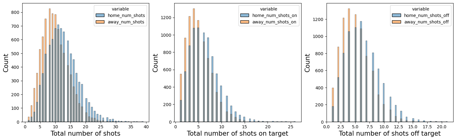
- The shape of the distribution of the home team and the away team is the same, but the distribution of the home team is shifted slightly to the right.
- It can be seen that the home teams took slightly more shots overall.
Q. Is there any difference of shot on target ratio(the number of shots on target / the number of shots) between home team and away team ?
home_away_shot_info["home_shot_on_target_ratio"] = home_away_shot_info.home_num_shots_on / home_away_shot_info.home_num_shots
home_away_shot_info["away_shot_on_target_ratio"] = home_away_shot_info.away_num_shots_on / home_away_shot_info.away_num_shots
home_away_shot_info["shot_on_target_ratio_difference"] = home_away_shot_info.home_shot_on_target_ratio - home_away_shot_info.away_shot_on_target_ratio
my_histogram(home_away_shot_info, "shot_on_target_ratio_difference")
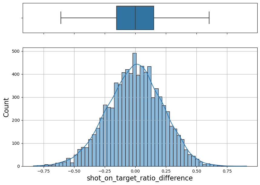
- Above plot shows the histogram of the shot on target ratio difference between the home team and the away team.
- There are also half of the matches where the away team had the higher shot on target ratio.
-
Since the distribution is symmetric, it is difficult to say that the home team had the particularly higher shot on target ratio than that of the away team.
- We have found that:
-
The number of shots and the number of shots on target have higher correlation with the number of goals than the number of shot off target
-
The shot on target ratio (the number of shots on target / total number of shots) have no difference between winning team and the losing team.
-
The shot on target ratio (the number of shots on target / total number of shots) have no difference between home team and the away team.
-
The winning teams usually have more shots, shots on target, and shots off target than those of the losing teams. $\$
-
The home teams usually have more shots, shots on target, and shots off target than those of the away teams. $\$
-
$\ \quad \rightarrow$ Of the three shot related variables(totla number of shots, number of shots on target, number of shots off target), consider only the total number of shots.
- Let’s check whether we can use the variables related to the number of shots for modeling.
df_match_ingame_shot_shot.match_api_id.drop_duplicates()
39980      489042
39992      489043
40006      489044
40021      489045
40033      489046
           ...
133702    2030168
133709    2030169
133714    2030170
133724    2030171
177951     499537
Name: match_api_id, Length: 8464, dtype: int64
df_match_basic.match_api_id.drop_duplicates()
0         492473
1         492474
2         492475
3         492476
4         492477
          ...
25974    1992091
25975    1992092
25976    1992093
25977    1992094
25978    1992095
Name: match_api_id, Length: 25979, dtype: int64
- Total number of matches: 25,979
- The number of matches that we have information about shots: 8,464 $\rightarrow$ That is, there are only 30% matches that have shots information. So it is hard to use the information related to the shots for training the model.
$\color{magenta} \quad \rightarrow$ So, we can show information related to number of shots into a dashboard later, but it is hard to use this information for modeling because there are too many matches that we don't have the shots information.
3. Summary
- Create a variable for each team that indicates how well they score goals when home, how well they block goals when home, how well they score goals when away, and how well they block goals when away:
- Each team’s last 1 / 3 / 5 / 10 / 20 / 30 / 60 / 90 matches
- average goal at home
- average opponent’s goal at home
- average goal at away
- average opponent’s goal at away
- Each team’s last 1 / 3 / 5 / 10 / 20 / 30 / 60 / 90 matches
-
Also, use the each team’s win or lose percentage at home and away for recent 1 / 3 / 5 / 10 / 20 / 30 / 60 / 90 matches.
- We can show information related to number of shots into a dashboard later, but it is hard to use this information for modeling because there are too many matches that we don’t have the shots information.